awvRfLoadPull

awvRfLoadPull(
w_waveform
[ ?maxValue x_maxValue ]
[ ?minValue x_minValue ]
[ ?numCont x_numCont ]
[ ?closeCont g_closeCont ]
[ ?name t_name ]
)
=> t / nil

Description

Draws load pull contour for the given waveform of PSS analysis. This function works only on two-dimensional sweep PSS results. The inner sweep must be phase and the outer sweep must be mag.

Arguments

w_waveform	Waveform of the signal.
?maxValue x_maxValue
	Largest value of the contour to be drawn. Default value is nil, which indicates that the largest value is to be taken from the results.
?minValue x_minValue
	Smallest value of the contour to be drawn. Default value is nil, which indicates that the smallest value is to be taken from the results.
?numCont x_numCont
	Number of points on the contour. Default values is 8.
?closeCont g_closeCont
	Specifies whether to draw a closed contour. Valid values are: t: Draws a closed contour. nil: Draws an open contour.
?name t_name	Name of the contour. Default value is p.

Value Returned

t	Load pull contour is drawn.
nil	Load pull contour cannot be drawn because of an error.

Examples

The following example creates a Waveform window and returns its window ID.

win1=awvCreatePlotWindow()

=> window:3

The following example opens the loadpull simulation results stored in the specified directory.

openResults("/home/user/loadpullsim/ExampleLibRF/lnaSimple/maestro/results/maestro/loadPULL/1/ExampleLibRF_lnaSimple_1/psf")

=>

"/home/user/loadpullsim/ExampleLibRF/lnaSimple/maestro/results/maestro/loadPULL/1/ExampleLibRF_lnaSimple_1/psf"

The following example lists the results available in the currently open results directory.

results()

(hb_mt_fi hb_mt_fd model instance output

    designParamVals primitives subckts variables

)

The following example selects the hb_mt_fi results from the results directory.

selectResults('hb_mt_fi)

=> stdobj@0x32b87cf8

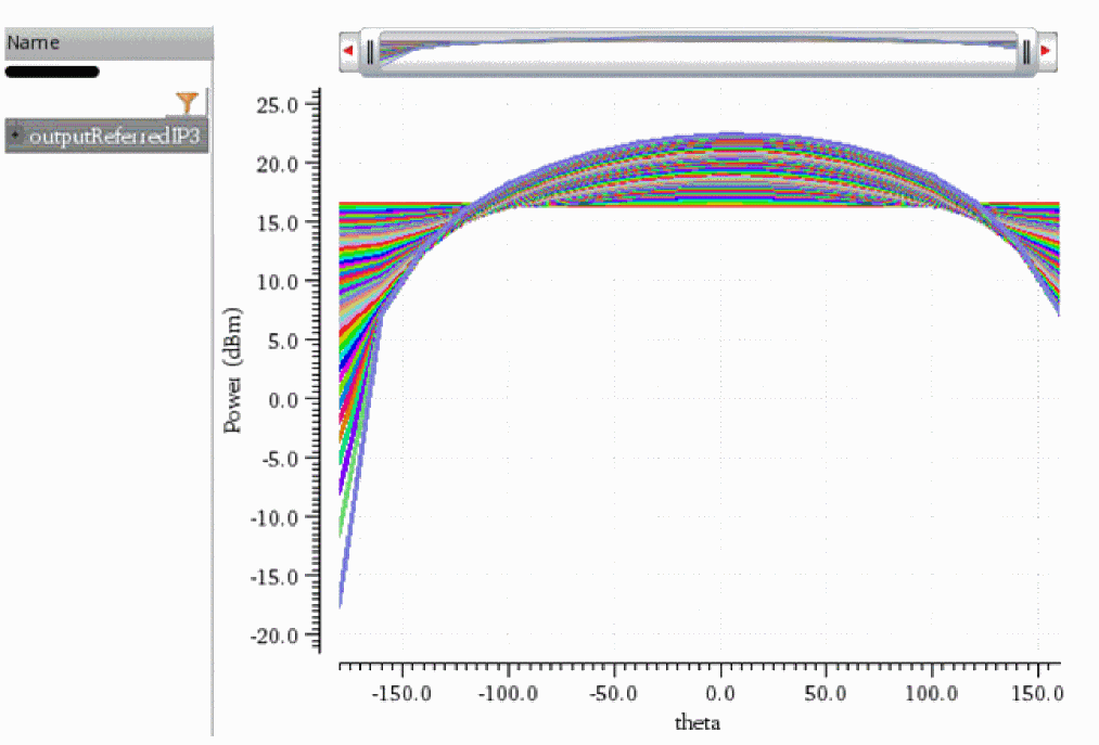
The following example creates a waveform object ip3, which represents the third-order intercept point (IP3) measurement done using two-tone harmonic balance analysis (hb_mt).

ip3=ipnVRI((v("/net047" ?result "hb_mt_fi") - 0.0) '(2 -1) '(0 1) ?rport resultParam("PORT0:r" ?result "hb_mt_fi") ?epoint -34 ?psweep nil ?measure "Output")

=> srrWave:0x3868af50

The following example plots the waveform object ip3 in the Waveform window win1.

awvPlotWaveform(

    win1

    list(ip3)

    ?expr list("outputReferredIP3")

    )

=> t

The following example creates another Waveform window and returns it window ID.

win2=awvCreatePlotWindow()

=> window:4

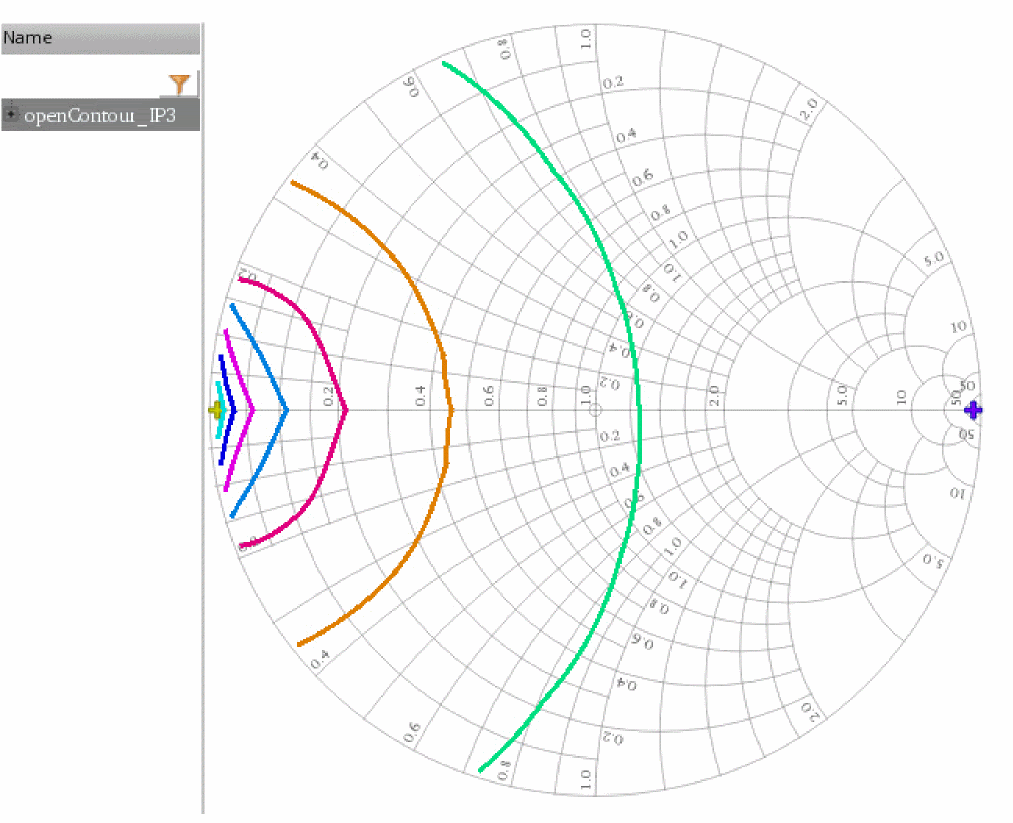
The following example sets display mode of the Waveform window win2 to smith.

awvSetDisplayMode(win2 "smith")

=> t

The following example sets the Smith display of the Waveform window win2 to impedance.

awvSetSmithModeType(win2 "impedance")

=> t

The following example creates a waveform object openContour, which represents 9 loadpull contours drawn for the input waveform ip3. In this example, note that the largest and smallest values of the contours are taken from the simulation results.

openContour=awvRfLoadPull(ip3 ?maxValue nil ?minValue nil ?numCont 9 ?closeCont nil)

=> srrWave:0x3868d5f0

The following example plots the waveform object openContour in the Waveform window win2.

awvPlotWaveform(

    win2

    list(openContour)

    ?expr list("openContour_IP3")

    )

=> t

The following example creates another Waveform window and returns it window ID.

win3=awvCreatePlotWindow()

=> window:5

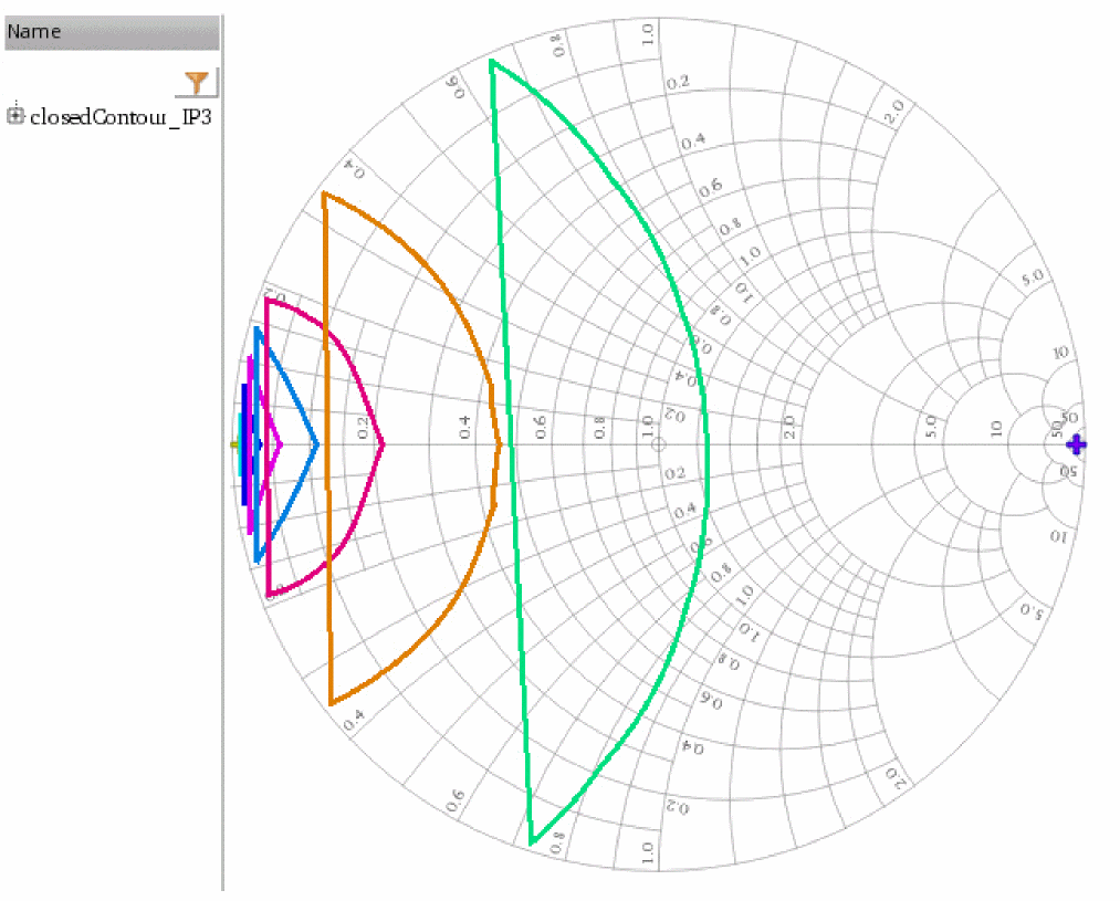
The following example sets display mode of the Waveform window win3 to smith.

awvSetDisplayMode(win3 "smith")

=> t

The following example sets the Smith display of the Waveform window win3 to impedance.

awvSetSmithModeType(win3 "impedance")

=> t

The following example creates a waveform object closedContour, which represents 9 loadpull contours drawn for the input waveform ip3. In this example, note that the largest and smallest values of the contours are taken from the simulation results.

closedContour=awvRfLoadPull(ip3 ?maxValue nil ?minValue nil ?numCont 9 ?closeCont t)

=> srrWave:0x3866d700

The following example plots the waveform object closedContour in the Waveform window win3.

awvPlotWaveform(

    win3

    list(closedContour)

    ?expr list("closedContour_IP3")

    )

=> t

Return to top