A

Built-In Functions

The built-in functions support two syntaxes:

Positional syntax
Requires each optional parameter up to and including the last optional parameter entered, but beyond that everything can be omitted.
```
cross( sig[, dir[, n[, thresh[, start[, xtol[, ytol[, accuracy]]]]]]] )
```

Named syntax
Allows any optional parameter to be specified — the preceding optional parameters need not be specified.

cross( sig=sig [, dir=dir] [, n=n] [, thresh=thresh] 
 [, start=start] [, xtol=xtol] [, ytol=ytol] 
 [, accuracy=accuracy] )

For example, the following statements are equivalent.

export real crossOut = cross(V(out), ’fall, 1, 1 )

export real crossOut = cross( sig=V(out), dir=’fall, n=1, thresh=1 )

abs

Returns the absolute value of a signal.

Syntax

abs( arg)

abs( arg=arg )

Arguments

arg

The scalar or signal.

Example

export real myabs = abs( -5 )

returns

myabs = 5

export real outabs = abs(arg=V(out))@1m

returns the value of the signal V(out) at 1ms.

acos

Returns the arc cosine of a signal.

Syntax

acos( arg )

acos( arg=arg )

Arguments

arg

The scalar or signal.

Example

export real myacos = acos( 1)

returns

myacos = 0

acosh

Returns the hyperbolic arc cosine of a signal.

Syntax

acosh( arg )

acosh( arg=arg )

Arguments

arg

The scalar or signal.

Example

export real myacosh = acosh( 1)

returns

myacosh = 0

analstop

Returns the simulation stop value.

Syntax

analstop( )

Arguments

None

Example

Used in MDL File

alias measurement transient {

run tran( step=1e-12, pstep=1e-12, stop=2e-08 )

export real anal_stop= analstop()

run  transient

returns

anal_stop = 2e-08

angle

Returns the angle of a real or complex number, or a waveform in degrees.

Syntax

angle( arg)

angle( arg=arg )

Arguments

arg

The real or complex number, or a waveform.

Example 1

export real myangle = angle( cplx(1,2) )

returns

myangle = 63.43

Example 2

export real phasemargin = angle( s(2,1) ) @ ft

returns

phasemargin= 15.0369

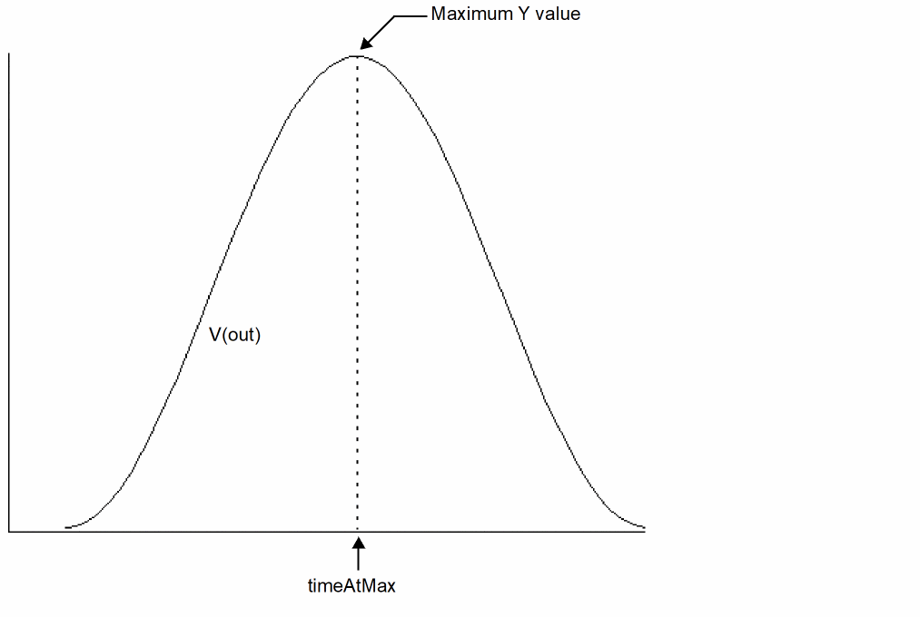
argmax

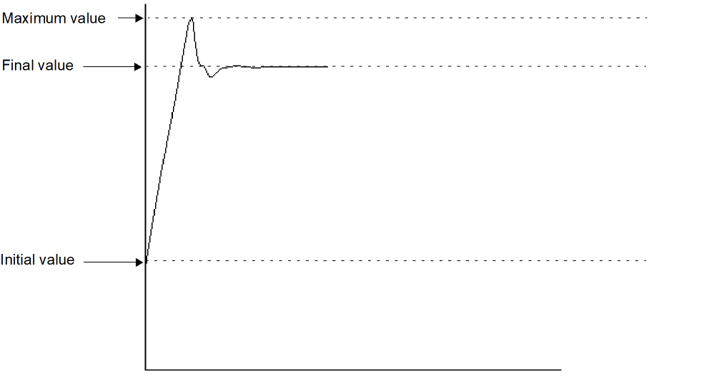
Returns the X value corresponding to the maximum Y value of a signal. If multiple X values are returned, the first one is used.

Syntax

argmax( sig )

argmax( sig=sig )

Arguments

sig

The signal.

Example

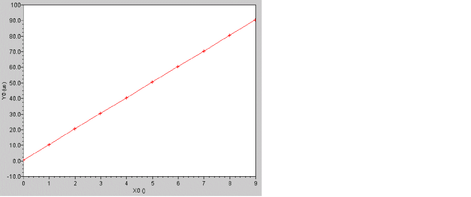
export real timeAtMax = argmax( V(out) )

The following diagram illustrates how the result is determined.

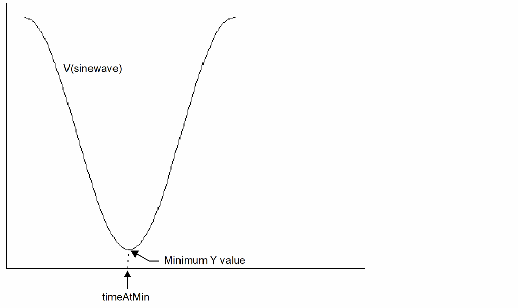
argmin

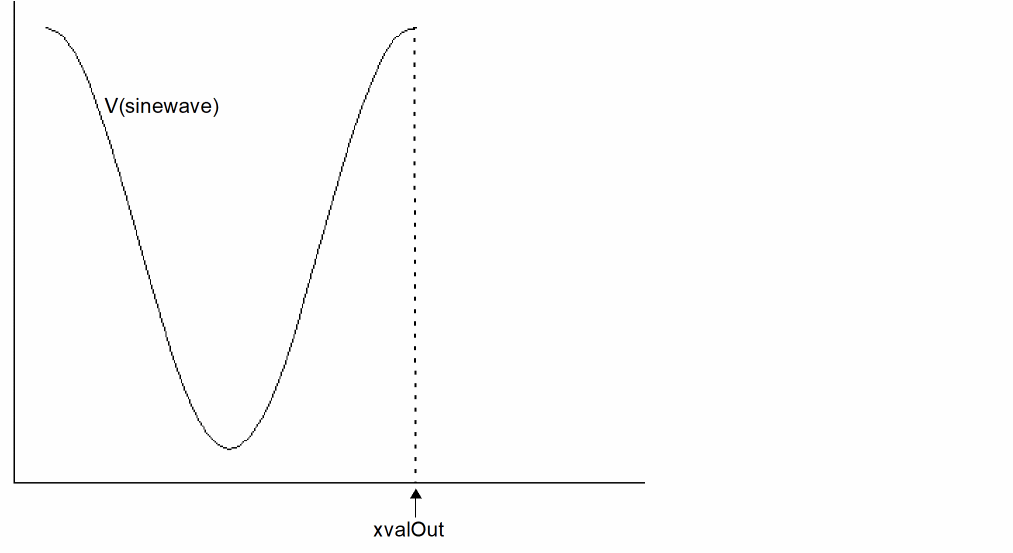
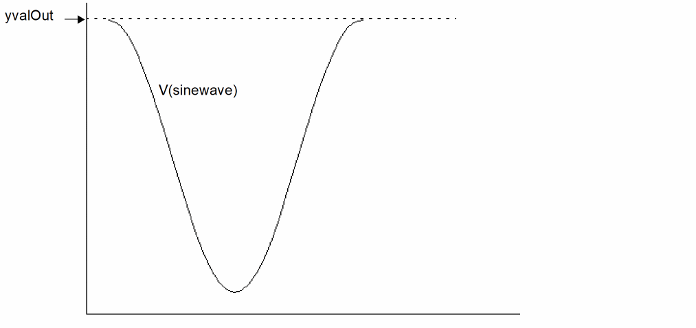
Returns the X value corresponding to the minimum Y value of a signal. If multiple X values are returned, the first one is used.

Syntax

argmin( arg )

argmin( arg=arg )

Arguments

arg

The signal.

Example

export real timeAtMin = argmin( V(sinewave) )

The following diagram illustrates how the result is determined.

asin

Returns the arc sine of a signal.

Syntax

asin( arg )

asin( arg=arg )

Arguments

arg

The scalar or signal.

Example

export real myasin = asin( 1 )

returns

myasin = 1.57

asinh

Returns the hyperbolic arc sine of a signal.

Syntax

asinh( arg )

asinh( arg=arg )

Arguments

arg

The scalar or signal.

Example

export real myasinh = asinh( 1 )

returns

myasinh = 0.88

atan

Returns the arc tangent of a signal.

Syntax

atan( arg )

atan( arg=arg )

Arguments

arg

The scalar or signal.

Example

export real myatan = atan( 1 )

returns

myatan = 1.56

atanh

Returns the hyperbolic arc tangent of a signal.

Syntax

atanh( arg )

atanh( arg=arg )

Arguments

arg

The scalar or signal.

avg

Returns the average value of a signal.

Syntax

avg( arg )

avg( arg=arg )

Arguments

arg

The signal.

Example

export real myavg = avg( V(out) )

avgdev

Returns the mean absolute deviation of a scalar argument or waveform. The mean absolute deviation is defined as follows:

1/N * ( |X1-mean| + |X2-mean| +...... |XN-mean| )

where | is the absolute value of the difference and N is the total number of Samples.

Syntax

avgdev( arg )

avgdev( arg=arg )

Arguments

arg

The scalar argument or waveform.

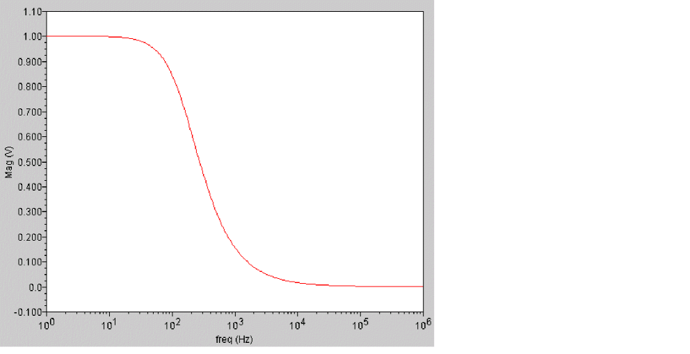
b w (bandwidth)

Calculates the bandwidth of a waveform.

Syntax

bw( sig, response, db, max )

bw( sig=sig, response=response, db=db, max=max )

Arguments

sig	The signal. In the SKILL mode, Virtuoso Visualization and Analysis XL wraps the signal with the `mag` function. In the MDL mode, you need to wrap the signal name with the `mag` function, otherwise Virtuoso Visualization and Analysis XL returns an error.
response	The response type: When `’low`, computes the low-pass bandwidth by determining the smallest frequency at which the magnitude of the input waveform drops db decibels below the DC gain. When `’high`, computes the high-pass bandwidth by determining the largest frequency at which the magnitude of the input waveform drops db decibels below the gain at the highest frequency in the response waveform. When `’band`, computes the band-pass bandwidth by: 1. Determining the lowest frequency (f`_max`) at which the magnitude of the input waveform is maximized; 2. Determining the highest frequency less than f`_max` at which the input waveform magnitude drops db decibels below the maximum; 3. Determining the lowest frequency greater than f`_max` at which the input waveform magnitude drops db decibels below the maximum; 4. Subtracting the value returned by step 2 from the value returned by step 3. The value returned by step 2 or step 3 must exist. Valid values: `’low`, `’high`, `’band`Default: `’low`
db	The decibels down from the peak. In the SKILL mode, db is a number equal to or greater than zero. In the MDL mode, db is a number less than zero. Default: -3.01029995664
max	The maximum amplitude of the waveform. You only need to specify this if you want to set the maximum amplitude lower than the waveform’s maximum value. If the max is specified, Measurement Description Language (MDL) uses this value instead of computing a value.

Example

Assume you have the following signal.

Then the following statement

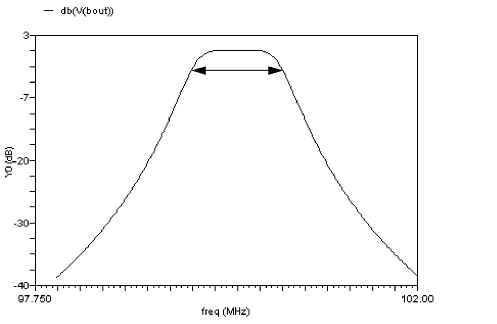
export real bwOut = bw(mag(V(bout)), response=’band)

generates, at the default db value of -3, the bw value

1000004.1627941281Hz

Note that the output in MDL includes the unit (Hz in the above example), whereas in SKILL it does not.

This value (approximately 1MHz) is illustrated on the graph by the double-ended arrow.

ceil

Rounds a real number up to the closest integer value.

Syntax

ceil( arg )

ceil( arg=arg )

Arguments

arg

The real number.

Example

export real myceil = ceil( 1.6 )

returns

myceil = 2

cfft

Performs a Fast Fourier Transform on a complex time domain waveform and returns its frequency spectrum. The cfft function takes two time signals that in combination form a complex input signal.

Syntax

cfft( sig_re, sig_im, from, to, numPoints[, window ])

cfft( sig_re=sig_re, sig_im=sig_im, from=from, to=to, numPoints=numPoints [, window=window ])

Arguments

sig_re	The real part of the signal.
sig_im	The imaginary part of the signal.
from	The starting X value.
to	The ending Y value.
numPoints	The number of data points to be used for calculating the cfft. If this number is not a power of 2, it is automatically raised to the next higher power of 2.
window	The algorithm used for calculating the cfft. In this release only one algorithm is supported. Valid value: `’rectangular`Default: `’rectangular`

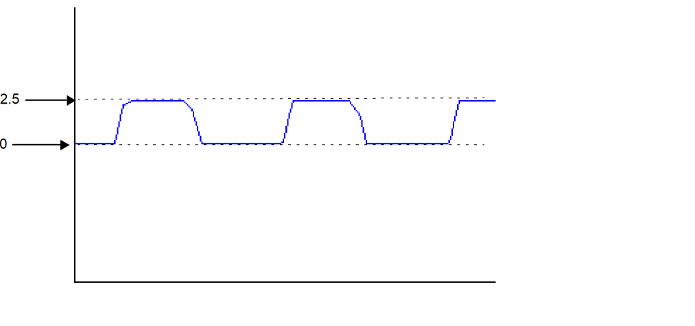
clip

Returns the portion of a signal between two points along the Y-axis.

Syntax

clip( sig, from, to )

clip( sig=sig, from=from, to=to )

Arguments

sig	The signal.
from	The starting point on the Y-axis.
to	The ending point on the Y-axis.

Example 1

The following example works in an MDL control file.

export real clipOut = avg ( clip (sig=V(sinewave), from=0, to=2.5) )

Example 2

In Virtuoso Visualization and Analysis XL,

clip (sig=V(sinewave), from=0, to=2.5)

transforms the following input signal

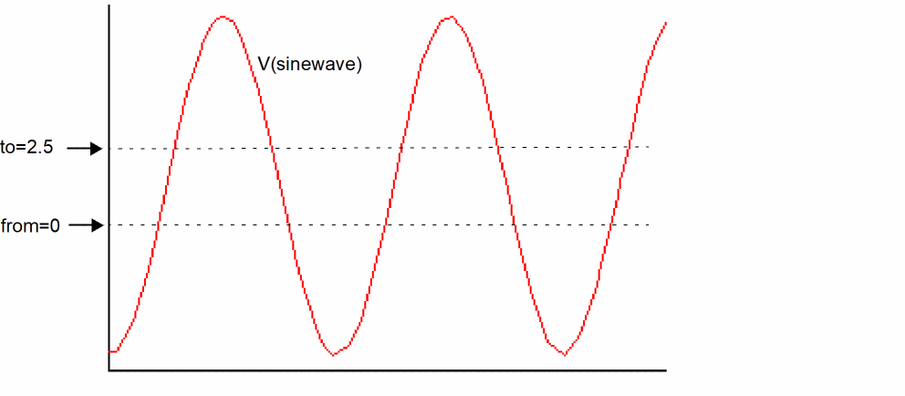
into the following output signal.

conj

Returns the conjugate of a complex number.

Syntax

conj( arg )

conj( arg=arg )

Arguments

arg

The complex number.

Example

export cplx mycplx = cplx ( 1,2 )
export cplx conj_mycplx = conj ( mycplx )

returns

mycplx = (1,2)
conj_mycplx = (1,-2)

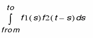
convolve

Returns a waveform consisting of the time domain convolution of two signals. This function is available in Virtuoso Visualization and Analysis XL only.

Syntax

convolve( sig1, sig2[, n_interp_steps ])

clip( sig1=sig1, sig2=sig2[, n_interp_steps=n_interp_steps ])

Arguments

sig1	The first signal.
sig2	The second signal.
n_interp_steps	Number of steps for interpolating waveforms.

Equation

Convolution is defined by the following equation:

Example

real vcdelay[]=crosses(sig=V(clock), thresh=0.9, dir='rise, n=1)
real outcross[]=crosses(V(q),n=6,thresh=vdd/2)
export real myconv[] = convolve(vcdelay,outcross,5)

returns

myconv[00]         =  2.57108e-13
myconv[01]         =  2.02971e-13
myconv[02]         =  1.74678e-13
myconv[03]         =  1.81539e-13
myconv[04]         =  2.03094e-13
myconv[05]         =  2.3083e-13
myconv[06]         =  2.65196e-13
myconv[07]         =  3.06643e-13
myconv[08]         =  3.55544e-13
myconv[09]         =  3.84546e-13
myconv[10]         =  3.94928e-13
myconv[11]         =  3.96003e-13
myconv[12]         =  3.88035e-13
myconv[13]         =  3.70677e-13
myconv[14]         =  3.43269e-13
myconv[15]         =  3.05072e-13

cos

Returns the cosine of a signal.

Syntax

cos( arg )

cos( arg=arg )

Arguments

arg

The scalar or signal.

Example

export real mycos = cos( 1 )

returns

mycos = 0.54

cosh

Returns the hyperbolic cosine of a signal.

Syntax

cosh( arg )

cosh( arg=arg )

Arguments

arg

The scalar or signal.

Example

export real mycosh = cosh( 1 )

returns

mycosh = 1.54

cplx

Returns a complex number created from two real arguments.

Syntax

cplx( R[, I] )

cplx( R=R [, I=I] )

Arguments

R	The value representing the real part.
I	The value representing the imaginary part.

Example

export cplx mycplx = cplx( 1,2 )

returns

mycplx = (1,2)

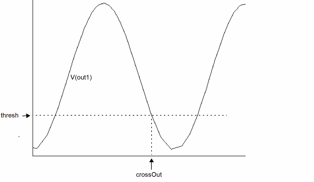
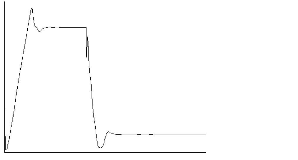
cross

Returns the X value where a signal crosses the threshold Y value.

Syntax

cross( sig[, dir[, n[, thresh[, start[, xtol[, ytol[, accuracy]]]]]]] )

cross( sig=sig[, dir=dir] [, n=n] [, thresh=thresh] [, start=start] [, xtol=xtol] [, ytol=ytol] [, accuracy=accuracy] )

Arguments

sig	The signal.
dir	The direction of the crossing event. `’rise` directs the function to look for crossings where the Y value is increasing, `’fall` for crossings where the Y value is decreasing, and `’cross` for crossings in either direction. Valid values: `’cross`, `’rise`, `’fall`Default: `’cross`
n	The occurrence of the crossing. The first crossing is n=1, the second crossing is n=2, and so on. The value of `n` can be negative numbers: n=-1 for the last occurrence before the end of the waveform, n=-2 for the second-last occurrence before the end of the waveform, and so on. Default: `1`
thresh	The threshold to be crossed. Default: `0`
start	The time at which the function is enabled. Default: `0`
xtol	The relative tolerance in percentage value in the X direction. Default: `1`
ytol	The relative tolerance in percentage value in the Y direction. Default: `1`
accuracy	Specifies whether the function should use interpolation, or use iteration controlled by the absolute tolerances to calculate the value. `’interp` directs the function to use interpolation, and `’exact` directs the function to consider the xtol and yval values. Data types: name for scalar Valid values: `’interp`, `’exact`Default: `’exact`

Example

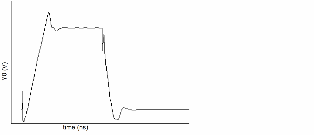
export real crossOut = cross( sig=V(out), dir=’fall, n=1, thresh=1 )

The following diagram illustrates how the result is determined.

crosscorr

Returns the cross correlation of the specified signals. This function is available only in Virtuoso Visualization and Analysis XL.

When the input signals are double waveforms,

crosscorr (sig1, sig2) = convolve (sig1, flip(sig2))

When one of the input signals is a complex waveform (sig2 in the following case),

crosscorr (sig1, sig2) = convolve (sig1, flip(conj(sig2)))

Syntax

crosscorr( sig1, sig2[, n_interp_steps ])

crosscorr( sig1=sig1, sig2=sig2[, n_interp_steps=n_interp_steps ])

Arguments

sig1	The first signal.
sig2	The second signal.
n_interp_steps	Number of steps for interpolating waveforms.

crosses

Returns the X values where a signal crosses the threshold Y value.

Syntax

crosses( sig[, dir[, n[, thresh[, start[, xtol[, ytol[, accuracy]]]]]]] )

crosses( sig=sig [, dir=dir] [, n=n] [, thresh=thresh] [, start=start] [, xtol=xtol] [, ytol=ytol] [, accuracy=accuracy] )

Arguments

sig	The signal.
dir	The direction of the crossing event. `’rise` directs the function to look for crossings where the Y value is increasing, `’fall` for crossings where the Y value is decreasing, and `’cross` for crossings in either direction. Valid values: `’cross`, `’rise`, `’fall`Default: `’cross`
n	The occurrence of the crossing. If n=1, the function returns the first crossing and all subsequent crossings. If n=3, the function returns the third crossing and all subsequent crossings. The value of n can be negative numbers: if n=-2, only the last two crossings are returned. Default: `1`
thresh	The threshold to be crossed. Default: `0`
start	The time at which the function is enabled. Default: `0`
xtol	The relative tolerance in percentage value in the X direction. Default: `1`
ytol	The relative tolerance in percentage value in the Y direction. Default: `1`
accuracy	Specifies whether the function should use interpolation, or use iteration controlled by the absolute tolerances to calculate the value. `’interp` directs the function to use interpolation, and `’exact` directs the function to consider the xtol and yval values. Data types: name for scalar Valid values: `’interp`, `’exact`Default: `’exact`

Example

export real crossesOut[] = crosses( sig=V(out), dir=’rise, thresh=0    .0 )

returns

crossesOut[0] = 1e-05

crossesOut[1] = 2e-05

crossesOut[2] = 3e-05

crossesOut[3] = 4e-05

crossesOut[4] = 5e-05

crossesOut[5] = 6e-05

crossesOut[6] = 7e-05

crossesOut[7] = 8e-05

crossesOut[8] = 9e-05

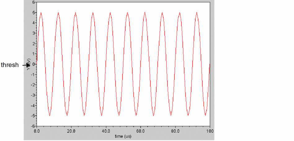
The output waveform looks as shown below:

d2r (degrees-to-radians)

Converts a waveform from degrees to radians.

Syntax

d2r( arg )

d2r( arg=arg )

Arguments

arg

The scalar or signal.

Example

export real myd2r = d2r( 180 )

db

Converts a signal to db where db=20*log(x). This function usually applies to voltage or current signals in volts or amperes.

Syntax

db( arg )

db( arg=arg )

Arguments

arg

The scalar or signal.

Example

export real dcgain = db( V(out) / V(in)) @1MHz

The above example assumes that out and in are signals from an ac dataset.

db10

Converts a signal to db where db=10*log(x). This function usually applies to power signals in watts.

Syntax

db10( arg )

db10( arg=arg )

Arguments

arg

The scalar or signal.

Example

export real mydb10= db10( v0:pwr )

dbm

Converts a signal to dbm where dbm=10*log(x)+30. This function usually applies to power signals in milliwatts (mW).

Syntax

dbm( arg )

dbm( arg=arg )

Arguments

arg

The scalar or signal.

Example

export real mydbm= dbm ( v0:pwr )

deltax

Returns the difference in the abscissas of two cross events.

Syntax

deltax( sig1[, sig2 [, dir1[, n1[, thresh1[, start1[, dir2[, n2[, thresh2[, start2], xtol[, ytol[, accuracy]]]]]]]]]]]] )

deltax( sig1=sig1, sig2=sig2 [, dir1=dir1] [, n1=n1] [, thresh1=thresh1] [, start1=start1] [, dir2=dir2] [, n2=n2] [, thresh2=thresh2] [, start2=start2] [, xtol=xtol][, ytol=ytol][, accuracy=accuracy])

Arguments

sig1	The signal whose cross event begins the measurement interval.
sig2	The signal whose cross event ends the measurement interval.
dir1	The direction of the cross at the beginning of the measurement interval. `’rise` directs the function to look for crossings where the Y value is increasing, `’fall` for crossings where the Y value is decreasing, and `’cross` for crossings in either direction. Valid values : `’cross` `’rise`, `’fall` Default: `’cross`
n1	The occurrence of the crossing for the beginning of the measurement interval. The first crossing is n=1, the second crossing is n=2, and so on. Default: `1`
thresh1	The Y value whose crossing begins the measurement interval. Default: 0
start1	The time at which the function is enabled. Default: 0
dir2	The direction of the cross at the end of the measurement interval. `’rise` directs the function to look for crossings where the Y value is increasing, `’fall` for crossings where the Y value is decreasing, and `’cross` for crossings in either direction. Valid values: `’cross`, `’rise`, `’fall` Default: `’cross`
n2	The occurrence of the crossing for the end of the measurement interval. The first crossing is n=1, the second crossing is n=2, and so on. Default: 1
thresh2	The Y value whose crossing ends the measurement interval. Default: 0
start2	The offset from `start1` where the function begins looking for the cross that ends the delay measurement. Default: 0
absstart2	The absolute offset from the beginning of the signal where the function begins looking for the cross that ends the delay measurement. Default: 0
xtol	The relative tolerance in percentage value in the X direction. Default: 1
ytol	The relative tolerance in percentage value in the Y direction. Default: 1
accuracy	Specifies whether the function should use interpolation, or use iteration controlled by the absolute tolerances to calculate the value. `’interp` directs the function to use interpolation, and `’exact` directs the function to consider the xtol and yval values. Data types: name for scalar Valid values: `’interp`, Default value: `’exact`

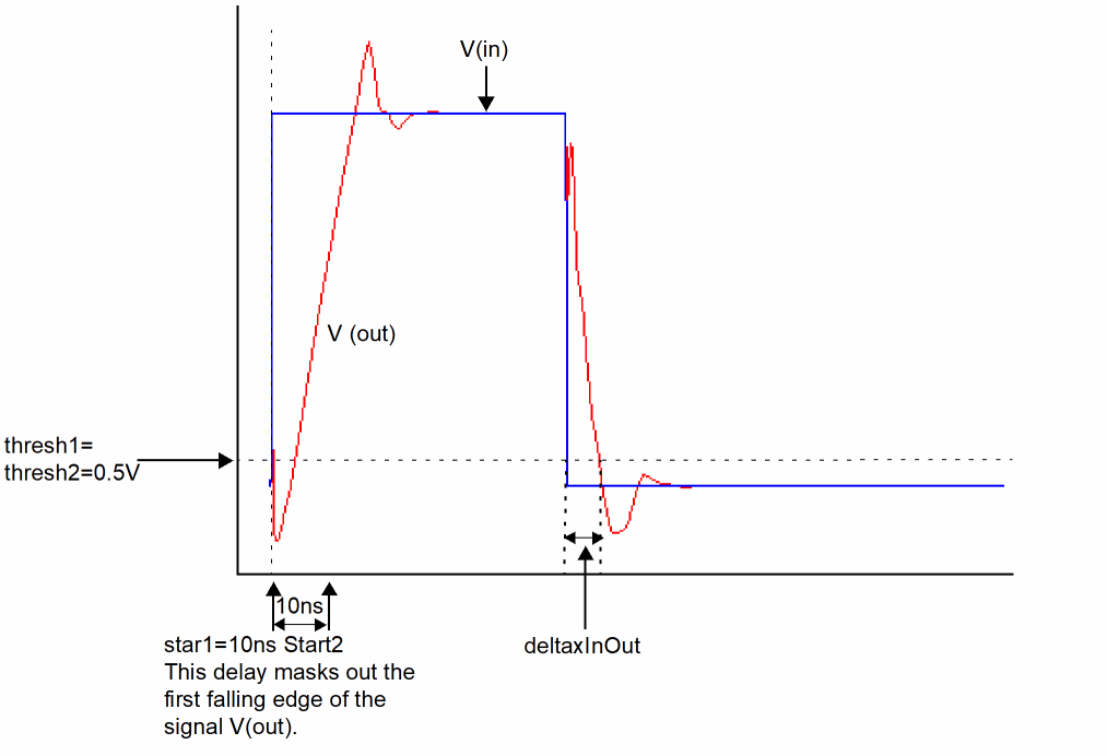
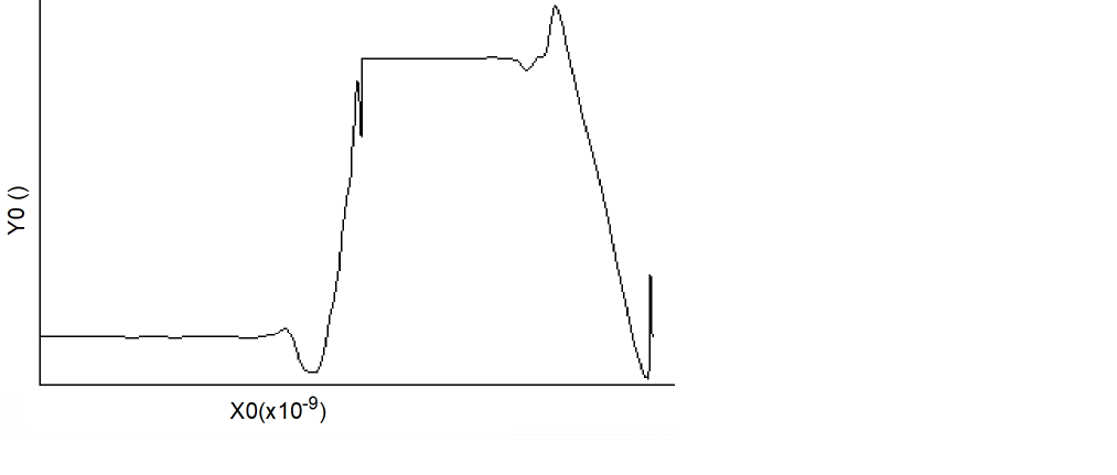
Example 1

export real deltaxInOut = deltax( sig1=V(in), sig2=V(out), dir1=’fall, \

thresh1 = 0.5, dir2=’fall, thresh2=0.5, start1=10n, start2=10n )

The following diagram illustrates how the result from the above example is determined.

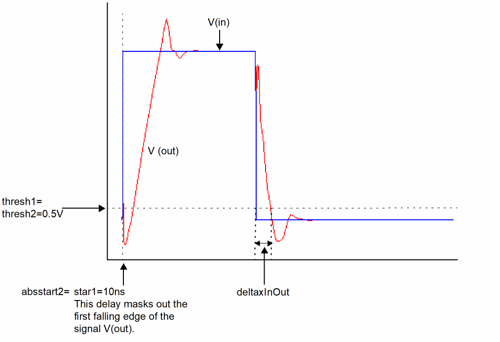
Example 2

export real delay2 = deltax( sig1=V(in), sig2=V(out), dir1=’fall, \

thresh1 = 0.5, dir2=’fall, thresh2=0.5, start1=10n, absstart2=10n )

The following diagram illustrates how the result from the above example is determined.

deltaxes

The deltaxes function is similar to the deltax function. However, it returns the differences in the abscissas of two cross events in the form of an array.

For syntax and arguments, please see deltax.

deriv

Returns the derivative of a signal.

Syntax

deriv( sig )

deriv( sig=sig )

Arguments

sig

The signal.

Example1

export real out_4n= deriv( V(out) )@4n

The derivative is calculated for signal V(out) at t=4ns.

Example 2

export real out_dvdt_fall=deriv(out)@cross(out, dir='fall, n=1, thresh=1.5)

The derivative is calculated for signal V(out) at its first crossing point at 1.5V in the fall direction.

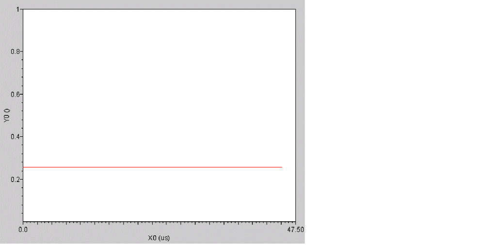
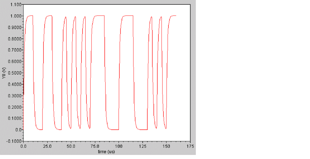
dutycycle

Calculates the ratio of the time for which the signal remains high to the period of the signal. You should use this function on periodic signals only.

Syntax

dutycycle( sig, theta, mode)

dutycycle( sig=sig, theta=theta, [ mode=’integrate |’percentage |’threshold ])

Arguments

sig	The signal.
theta	Percentage that defines the logic high of the signal. A threshold value is calculated as follows: yThresh=((Ymax - Ymin) * theta * 0.01) + Ymin The portion of the signal above yThresh is taken as high. Default value: `50.0`
mode=’integrate	If `mode` is set to `integrate`, `theta` is ignored and the threshold value is calculated as in the SKILL mode.
mode=’percentage	If `mode` is set to `percentage`, `theta` will be a percentage value. This is the default value.
mode=’threshold	If `mode` is set to `threshold`, the value of `theta` is taken as the threshold value.

If mode is not specified, it will automatically be set to percentage.

Example

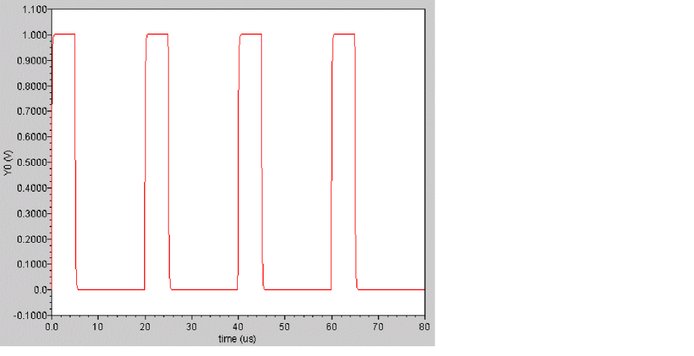
export real dutycycleOut = dutycycle ( sig=V(out), theta=40 )

returns

dutycycleOut = 0.25436626860397216

dutycycles

Returns the dutycycle of a nearly-periodic signal as a function of time.

Syntax

dutycycles( sig, theta )

dutycycles( sig=sig, theta=theta )

Arguments

sig

The signal.

theta

Percentage that defines the logic high of the signal. A threshold value is calculated as follows:

yThresh=((Ymax - Ymin) * theta * 0.01) + Ymin

The portion of the signal above yThresh is taken as high. Default value: 50.0

Example 1

In Virtuoso Visualization and Analysis XL,

export real dutycyclesOut = dutycycles ( sig=V(out), theta=40 )

Example 2

export real dutycycles_q[] = dutycycles ( sig=V(q), theta=40 )

returns

dutycycles_q[0] = 0.3877

dutycycles_q[1] = 0.6897

dutycycles_q[2] = 0.685696

transforms the following input signal

into the following output signal

exp

Returns the e^x value of a signal.

Syntax

exp( arg )

exp( arg=arg )

Arguments

arg

The scalar or signal.

Example

export real myexp = exp( 2 )

returns

myexp = 7.389

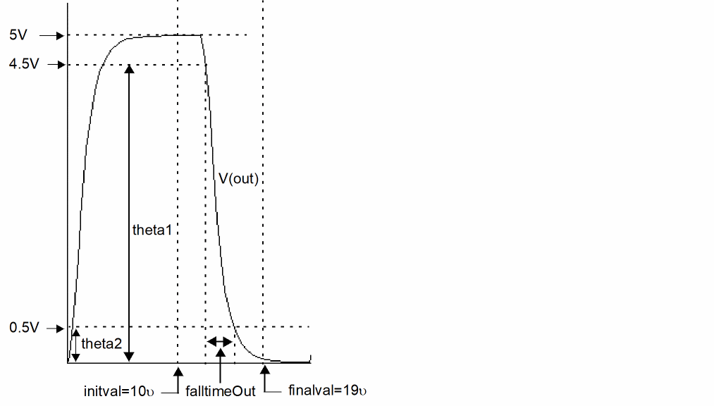
falltime

Returns the fall time for a signal measured between percent high and percent low of the difference between the initial and final values. The measurement is always done with ordinate (Y-axis) values.

You can use the falltimes function to obtain the fall time for all edges instead of a single edge that is returned by the falltime function.

Syntax

falltime( sig[, initval[, finalval[, inittype[, finaltype[, theta1[, theta2[, xtol[, ytol[, accuracy]]]]]]]]] )

falltime( sig=sig, initval=initval, finalval=finalval [, inittype=inittype] [, finaltype=finaltype] [, theta1=theta1] [, theta2=theta2] [, xtol=xtol] [, ytol=ytol] [, accuracy=accuracy] )

Arguments

sig	The signal.
initval	The Y-axis value (if inittype is `’y`) or X-axis value at the specified X-axis point (if inittype is `’x`) that starts the falltime interval.
finalval	The Y-axis value (if inittype is `’y`) or X-axis value at the specified X-axis point (if inittype is `’x`) that ends the falltime interval.
inittype	When `’x`, the initial value is an X value. When `’y`, the initial value is a Y value. Valid values: `’x, ’y` Default: `’y`
finaltype	When `’x`, the final value is an X value. When `’y`, the final value is a Y value. Valid values: `’x, ’y` Default: `’y`
theta1	The threshold high expressed as a percentage of the difference between the initial and final values. Default: `90`
theta2	The threshold low expressed as a percentage of the difference between the initial and final values. Default: `10`
xtol	The relative tolerance in percentage value in the X direction. Default: `1`
ytol	The relative tolerance in percentage value in the Y direction. Default: `1`
accuracy	Specifies whether the function should use interpolation, or use iteration controlled by the absolute tolerances to calculate the value. `’interp` directs the function to use interpolation, and `’exact` directs the function to consider the xtol and yval values. Data types: name for scalar Valid values: `’interp`, `’exact` Default: `’exact`

Example

export real falltimeOut = falltime ( arg=V(out), initval=10u, inittype=’x, finalval=19u, finaltype=’x, theta1=90, theta2=10)

The following diagram illustrates how the result from the above example is determined.

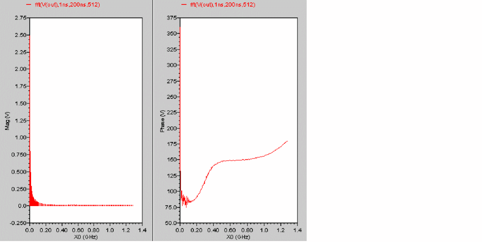
fft

Performs a Fast Fourier Transform on the signal and returns its frequency spectrum.

Syntax

fft( sig, from, to, numPoints, window )

fft( sig=sig, from=from, to=to, numPoints=numPoints, window=window )

Arguments

sig	The signal.
from	The starting X value.
to	The ending X value.
numPoints	The number of data points to be used for calculating the fft. If this number is not a power of 2, it is automatically raised to the next higher power of 2.
window	The algorithm used for calculating the fft. For more information, see window. Valid values: `’rectangular`, `’bartlett`, `’bartletthann`, `’blackman`, `’blackmanharris`,`’cosine2`, `’cosine4`, `’extcosbell`, `’flattop`, `’halfcyclesine`, `’half3cyclesine`, `’halfcyclesine3`, `’half6cyclesine`, `’halfcyclesine6`, `’hamming`, `’hanning`, `’nuttall`, `’parzen`, `’triangular` Default: `’rectangular`

Example

In Virtuoso Visualization and Analysis XL,

fft( sig=(V(out), from=1ns, to=200ns, numPoints=512, window=’bartlett)

transforms the following input signal

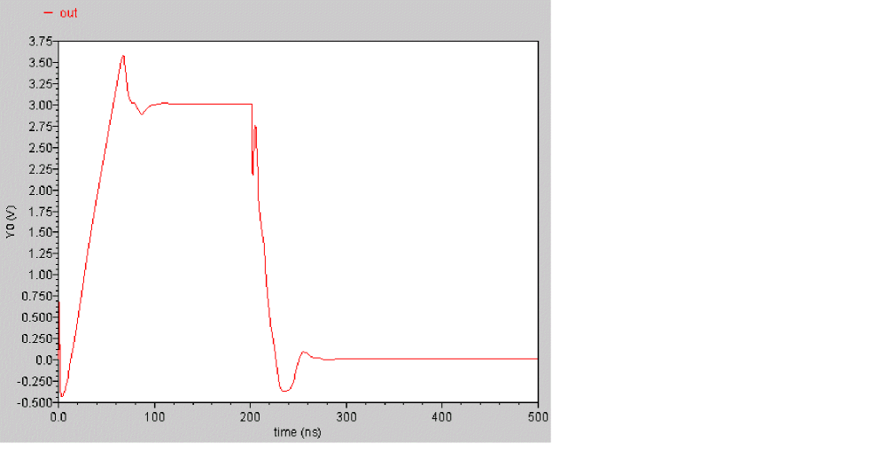
into the following output signal. The left subwindow shows the magnitude part of the spectrum and the right subwindow shows the phase part.

flip

Returns a reversed version of a signal (rotates the signal along the Y-axis).

Syntax

flip ( sig )

flip( sig=sig )

Arguments

sig

The signal.

Example

export real flipOut = flip( V(out) )

transforms the following input signal

into the following output signal.

floor

Rounds a real number down to the closest integer value.

Syntax

floor( arg )

floor( arg=arg )

Arguments

arg

The real number.

Example

export real myfloor = floor( 1.6 )

returns

myfloor = 1

fmt

Provides formatting capability to turn MDL datatypes into a string representation.

Syntax

fmt( “format”, varargs )

fmt( format=”format”, varargs=varargs )

Arguments

“format”

The percent code format string. In addition to the standard percent codes in C ( %s, %S, %g, %G, %e, %E, %f, %d, %i, %u, %o, %x, %X), the following percent codes are also available:
%V - the value of the varargs argument.
The following “\” qualifiers (constant escape sequences) are also supported:
\n - newline
\t - tab
In addition to these, full precision qualifier support exists for all supported percent codes.

varargs

Arguments to the fmt function used to fill in the percent code values in the format string.

Example

alias measurement printmeas {
    input string out="myfile.out"
    print fmt("Header is %s\n", out) to=out
    print fmt("%s\t%s\t\t%s\t%s\t%s\t%s\n", 
     "%d","%f","%o","%x","%X","%u") addto=out
 print fmt("%d\t%f\t%o\t%x\t%X\t%u\n",10,10,10,10,10,10) addto=out

run printmeas (out="test.dat")

The simulator writes the following results to the test.dat file:

Header is test.dat

%d      %f              %o      %x      %X      %u

10      10.000000       12      a       A       10

freq

Returns an array of frequencies defined by the given threshold crossing and direction for a signal.

Syntax

freq( sig, thresh, dir )

freq( sig=sig, thresh=thresh, dir=direction )

Arguments

sig

The signal.

thresh

The threshold Y-axis value to be crossed.

dir

The direction of the crossing event.

Valid values: ’rise, ’fall

Example

In Virtuoso Visualization and Analysis XL,

export real freqOut = freq ( sig=V(out), thresh=0.5, dir=’rise )

returns

freqOut[0] = 5.0001e+04

freqOut[1] = 5e+04

the following input signal

is converted to the following output signal

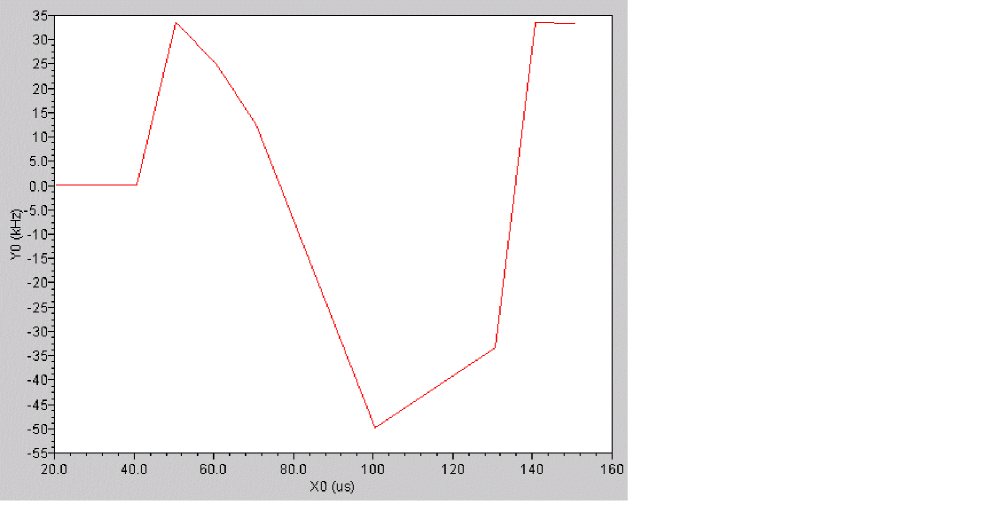
freq_jitter

Returns a waveform representing the deviation from the average frequency.

Syntax

freq_jitter( sig, thresh, dir, binsize )

freq_jitter( sig=sig, thresh=thresh, dir=direction, binsize=binsize )

Arguments

sig	The signal.
thresh	The threshold Y-axis value to be crossed.
dir	The direction of the crossing event. Valid values: `’rise`, `’fall`
binsize	Integer used to calculate the average frequency of the signal. If binsize=0, all frequencies are used to calculate the average. If binsize=N, the last N frequencies are used to calculate the average. Default value=`0`

Example

In Virtuoso Visualization and Analysis XL,

export real freq_jitterOut = freq_jitter ( sig=V(out), thresh=0.5, dir=’rise, binsize=4 )

the following input signal

is converted to the following output signal

gainBwProd

Returns the product of DC gain and upper cutoff frequency for a low-pass type filter or amplifier.

Syntax

gainBwProd( sig )

gainBwProd( sig=sig )

Arguments

sig

The signal. It can represent the magnitude of the gain or a frequency response.

Example

export real gainBwProdOut = gainBwProd ( sig=mag(out) )

returns

gainBwProdOut = 1804641.158689868

gainmargin

Computes the gain margin of the loop gain of an amplifier.

The gain margin is calculated as the magnitude (in dB) of the gain at f0. The frequency f0 is the smallest frequency in which the phase of the gain provided is -180 degrees. For stability, the gain margin must be positive.

Syntax

gainmargin( sig )

gainmargin( sig=sig )

Arguments

sig

The loop gain of interest over a sufficiently large frequency range.

Example

export real gainmar=gainmargin(vout)

getinfo

Returns information related to the simulator, such as version, subversion, and command information.

Syntax

getinfo( type )

getinfo( type=type )

Arguments

type

Type of information to be displayed. Valid values are ’simulator, ’version, ’subversion, and ’cmd.

Example

string simulator=getinfo(’simulator)

string version=getinfo(’version)

string subversion=getinfo(’subversion)

string cmdline=getinfo(’cmd)

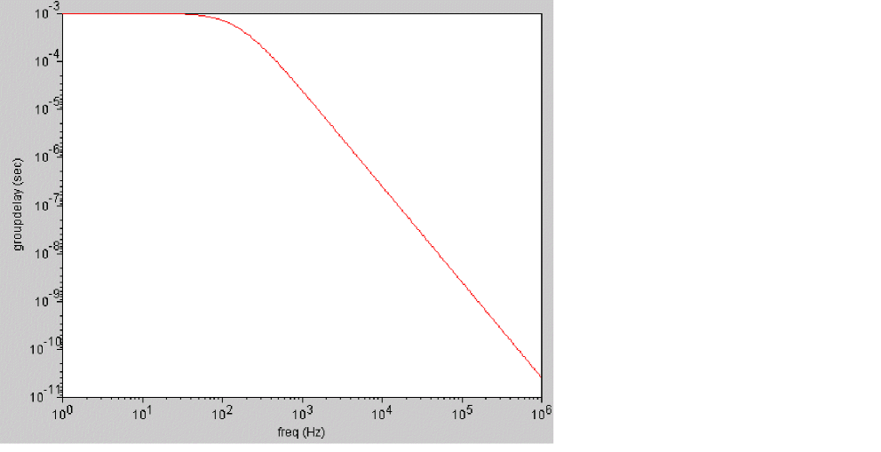
groupdelay

Calculates the rate of change of phase with respect to frequency in a frequency response measurement.

groupdelay=d(phase)/dw

where w=angular frequency in rad/s=2*PI*f

Syntax

groupdelay( sig )

groupdelay( sig=sig )

Arguments

sig

The signal. It should represent frequency response.

Example

In Virtuoso Visualization and Analysis XL,

export real groupdelayOut = groupdelay ( sig=out )

the following input signal

is converted to the following output signal

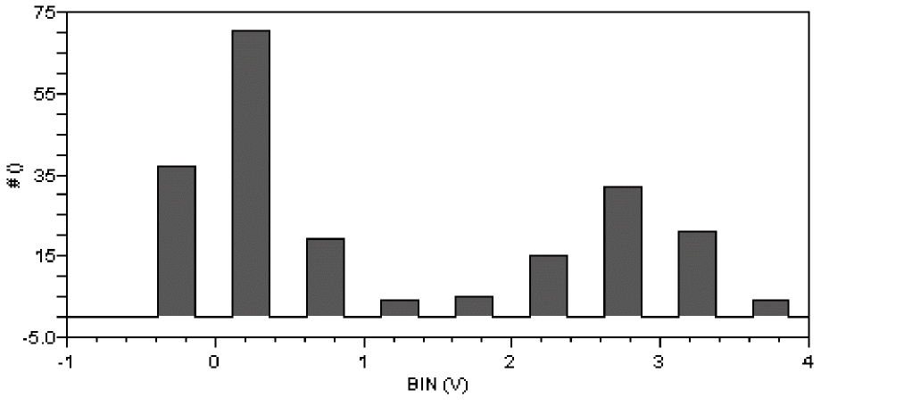
histo

Creates a histogram from a signal.

The histo function is available from the calculator. It is not supported within a Spectre MDL control file since it returns a scalar and not a waveform.

Syntax

histo( sig, nbins, min, max )

histo( sig=sig, nbins=nbins, min=min, max=max )

Arguments

sig	The waveform.
nbins	The number of bins to be created.
min	The value that specifies the smaller end point of the range of values included in the histogram.
max	The value that specifies the larger end point of the range of values of values included in the histogram.

Example

histo(V(out),nbins=10, min=-1.0, max=4.0)

creates a display with 10 bins that might look like this when the leftmost bin is empty.

I

Current probe function.

Syntax

I(devname)     //equivalent to devname:0

I(devname:term)     //term can be either terminal name or terminal index

I(Instname:term)     //term can be either terminal name or terminal index

The I probe function does not support current access by node name, nor does it support current difference between two devname:term(s). In other words, it is illegal to apply the I probe to a node or a pair of nodes.

Arguments

devname	The N-terminal device instance name.
Instname	The N-terminal subcircuit instance name.
term	The terminal name or terminal index of a device or a subcircuit.

Examples

I(Rload:1)    // Returns the current through terminal Rload:1

I(I0.mp1:d)   // Returns the current through device terminal name d

I(I0:vdd1)    // Returns the current through subcircuit terminal name vdd1

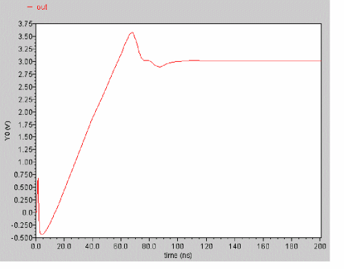
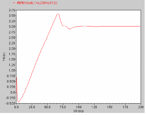
ifft

Performs an inverse Fast Fourier Transform on a frequency spectrum and returns the time domain representation of the spectrum.

Syntax

ifft ( sig )

ifft( sig=sig)

Arguments

sig

The frequency spectrum.

Example

fft( sig=V(out), from=1ns, to=200ns, npoints=512)

results in the graph on the right side.

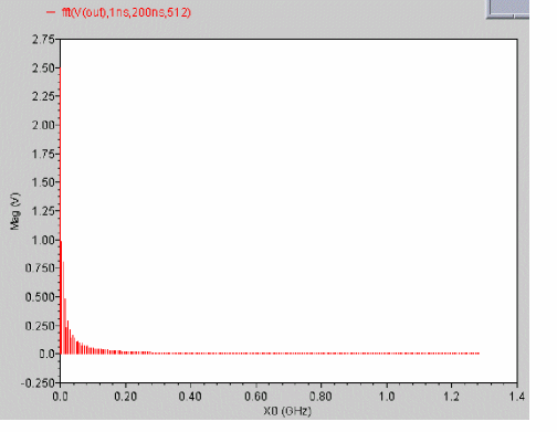The signal `out`	Fast fourier transform of the signal `out`

Now if I perform an ifft on the above expression,

ifft( fft( sig=V(out), from=1ns, to=200ns, npoints=512) )

The result is the same as the original signal (out) – from 1ns to 200ns.

iinteg

Returns the incremental area under the waveform.

Syntax

iinteg( sig )

iinteg( sig=sig )

Arguments

sig

The signal.

Example 1

export real iintegOut = iinteg( V(out) )

transforms the following input signal

into the following output signal

Each X value on the output trace is equal to the area under the input trace from start till that particular X-value.

im

Returns the imaginary part of a complex number.

Syntax

im( arg )

im( arg=arg )

Arguments

arg

The complex number.

Examples

export real myim = im( cplx(1,2) )

returns

myim = 2

export real im_sll = im( s(1,1) )

returns

im_sll = 0.670029

int

Returns the integer portion of a real value.

Syntax

int( arg )

int( arg=arg )

Arguments

arg

The real number whose integer portion is to be returned.

Example

int(4.998)

returns the value

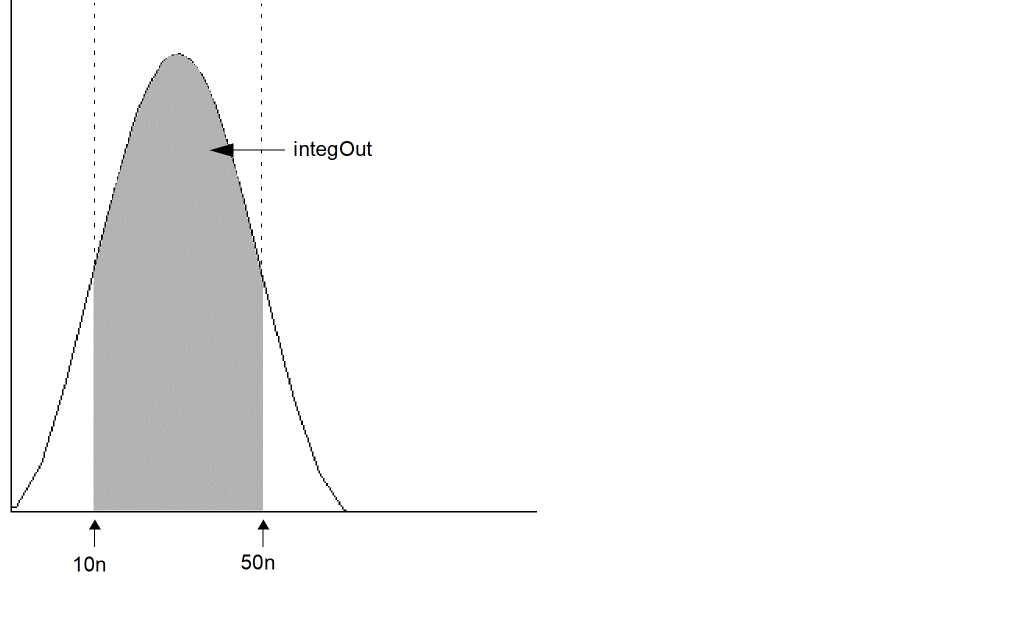
integ

Returns the area bounded under the curve.

Syntax

integ( sig )

integ( sig=sig )

Arguments

sig

The signal.

Example 1

export real integOut = integ( trim( sig=V(sinewave), from=10n, to=50n ) )

The following diagram illustrates how the result from the above example is determined. The result is equal to the shaded area in the graph.

ln

Returns the natural logarithm of a signal or a number. If no specific point of a signal is specified, MDL returns value for the last simulation point of the signal.

Syntax

ln( arg )

ln( arg=arg )

Arguments

arg

The scalar or signal.

Examples

export real mylog = ln ( 10 )

returns

mylog = 2.3

export real myln = ln ( v(q))

export real myln_ons = ln ( v(q) @0 )

returns

myln     = -0.223144

myln_ons       = -21.9773

log10

Returns the base 10 logarithm of a signal or a number. If no specific point of a signal is specified, MDL returns value for the last simulation point of the signal.

Syntax

log10( arg )

log10( arg=arg )

Arguments

arg

The scalar or signal.

Example

export real mylog10 = log10( 10 )

returns

mylog10 = 1

mag

Returns the magnitude of a signal or complex number.

Syntax

mag( arg )

mag( arg=arg )

Arguments

arg

The scalar or signal.

Example

export real mymag = mag( cplx(1,2) )

returns

mymag = 2.236

max

Returns the maximum value of a signal, maximum value of two real values, or the maximum value or a signal and a real value

Syntax

max( arg )

max( arg=arg )

Arguments

arg

The scalar or signal.

Example 1

export real maxOut1 = max ( V(out ) )

Example 2

export real maxOut2 = max ( V(out)@100n, V(out)@200n )

This returns the value of out at 100n or 200n – whichever is greater.

Example 3

export real maxq=max(trim(q, from=0, to=100n))

This returns the maximum value of out over the range of t=0ns to t=100ns.

Example 4

export real maxOut4 = max( I(IP1)@ 1.0 , 1e-15 );

min

Returns the minimum value of a signal or the minimum value of two real values.

Syntax

min( arg )

min( arg=arg )

Arguments

arg

The scalar or signal.

Example

export real minOut1 = min( V(out) )

Example 2

export real minOut2 = min ( V(out)@100n, V(out)@200n )

This returns the value of out at 100n or 200n – whichever is smaller.

mod

Returns the floating point remainder of the dividend divided by the divisor. The divisor cannot be zero.

Syntax

mod( dividend, divisor )

mod( dividend=dividend, divisor=divisor )

Arguments

dividend	The scalar dividend.
divisor	The scalar divisor.

Example

export real mymod = mod( 546, 324 )

returns

mymod = 222

movingavg

Calculates the moving average for the specified signal.

Syntax

movingavg( sig[, n ])

movingavg( sig=sig[, n=n ] )

Arguments

sig

The signal.

Number of points specifying the bin size.

Default: 1

overshoot

Returns the overshoot/undershoot of a signal as a percentage of the difference between initial and final values.

Syntax

overshoot( sig[, initval[, finalval[, inittype[, finaltype]]]] )

overshoot( sig=sig, initval=initval, finalval=finalval [, inittype=inittype] [, finaltype=finaltype] )

Arguments

sig	The signal.
initval	The initial value. To calculate the undershoot of a signal, the initval should be higher than finalval.
finalval	The final value.
inittype	When `’x`, the initial value is a time value. When `’y`, the initial value is a current or voltage value. Valid values: `’x, ’y` Default: `’y`
finaltype	When `’x`, the final value is a time value. When `’y`, the final value is a current or voltage value. Valid values: `’x, ’y` Default: `’y`

Example

export real overshootOut = overshoot ( sig=V(out), initval=1, finalval=3, inittype=’y, finaltype=’y) )

OvershooutOut is given by the following formula:

period_jitter

Returns a waveform representing the deviation from the average period.

Syntax

period_jitter( sig, thresh, dir, binsize )

period_jitter( sig=sig, thresh=thresh, dir=direction, binsize=binsize )

Arguments

sig	The signal.
thresh	The threshold Y-axis value defining the period/frequency of the signal.
dir	The direction of the crossing event. Valid values: `’rise`, `’fall` Default value: `’rise`
binsize	Integer used to calculate the average frequency of the signal. If binsize=0, all periods are used to calculate the average. If binsize=N, the last N periods are used to calculate the average. Default value=`0`

Example

export real period_jitterOut = period_jitter ( sig=V(out), thresh=0.5, dir=’rise, binsize=4 )

ph

Returns the phase of a signal in radians.

Syntax

ph( arg[, wrap=<value> ])

ph( arg=arg, wrap=value )

Arguments

arg	The signal.
`value`	Wraps the phase. The phase is wrapped around +/- PI. Possible values are `yes` (default) and `no`. The value can be scalar.

Example

ph( v(out), wrap=’no )

phasemargin

Computes the phase margin of the loop gain of an amplifier. The phase margin is calculated as the difference between the phase of the gain in degrees at f0 and at -180 degrees. The frequency f0 is the smallest frequency where the gain is 1. For stability, the phase margin must be positive. The value is returned in degrees.

Syntax

phasemargin( sig )

phasemargin( sig=sig )

Arguments

sig

The loop gain of interest over a sufficiently large frequency range. sig can be v(nodeName) or I(deviceName).

Example

export real phasemar=phasemargin(vout)

pow

Returns the value of base raised to the power of exponent (baseexponent).

Syntax

pow( base, exponent )

pow( base=base, exponent=exponent )

Arguments

base	The base argument.
exponent	The exponent argument.

Example

export real mypow = pow( 2,2 )

returns

mypow = 4

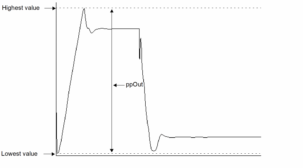
pp (peak-to-peak)

Returns the difference between the highest and lowest values of a signal.

Syntax

pp( sig)

pp( sig=sig )

Arguments

sig

The signal.

Example 1

export real ppOut = pp( V(out) )

The following diagram illustrates how the result from the above example is determined.

pzbode

Calculates and plots the transfer function for a circuit from pole zero simulation data. This function is available only in the MDL mode.

Syntax

pzbode( poles, zeroes, c, minfreq, maxfreq, npoints)

pzbode( poles=poles , zeroes=zeroes , c=c , minfreq=minfreq , maxfreq=maxfreq , npoints=npoints )

Arguments

poles	The poles.
zeroes	The zeroes.
c	The transfer gain constant.
minfreq	The minimum frequency for the bode plot.
maxfreq	The maximum frequency for the bode plot.
npoints	The frequency interval for the bode plot, in points per decade.

Example

The following diagram illustrates how the result with the values poles=POLES‹I‹R_1››, zeroes=ZEROES‹I‹R_1››, c=I‹R_1›\[K\], minfreq=1e-3, maxfreq=1e3, and npoints=1000 is determined.

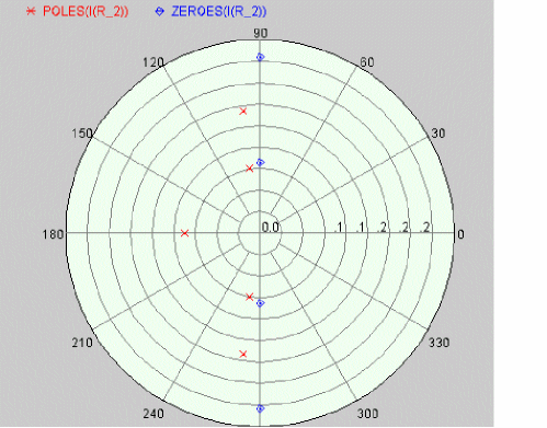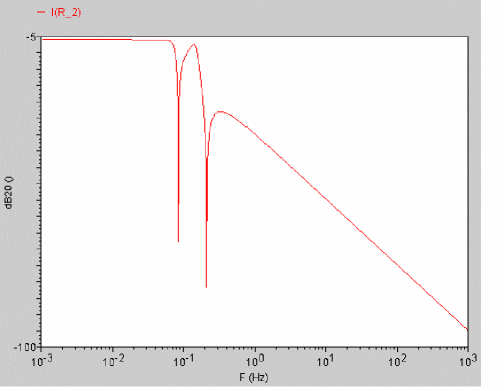Polar Plot	Corresponding bode plot

pzfilter

Filters the poles and zeroes according to the specified criteria. The pzfilter function works only on pole zero simulation data. This function is available only in the MDL mode.

Syntax

pzfilter( poles, zeroes, maxfreq, reldist, absdist, minq)

pzfilter( poles=poles , zeroes=zeroes , maxfreq=maxfreq , reldist=reldist , absdist=absdist , minq=minq )

Arguments

poles	The poles.
zeroes	The zeroes.
maxfreq	The frequency up to which the poles and zeroes are plotted.
reldist	The relative distance between the pole and zero. Pole-zero pairs with a relative distance lower than the specified value are not plotted.
absdist	The absolute distance between the pole and zero. Pole-zero pairs with an absolute distance lower than the specified value are not plotted.
minq	The minimum Q-factor. Pole-zero pairs with a Q-factor less than the specified value are not cancelled. The equations that define the Q-factor of a complex pole or zero are described in the section below.

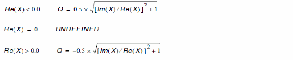
If you do not specify maxfreq, reldist, absdist, or minq, pzfilter filters out the poles and zeroes with a frequency higher than 10 GHz (default value of maxfreq).

Equations Defining the Q-Factor of a Complex Pole or Zero

Filtration Rules

Real poles can be cancelled only by real zeroes. A real pole P is cancelled by a real zero Z if the following equation is satisfied:
Complex poles and zeroes always occur in conjugated pairs. A pair of conjugated poles can only be canceled by a pair of conjugated zeroes. A pole pair P1=a+jb, P2=a-jb is cancelled by a zero pair Z1=c+jd, Z2=c-jd, if the following equation is satisfied:
Poles in the right-half plane are never cancelled because they show the instability of the circuit.

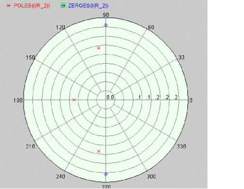
Example

The values poles=POLES‹I‹R_2››, zeroes=ZEROES‹I‹R_2››, absdist=0.05, and minq=10000 filters pole-zero pairs with a relative distance of less than 0.05 Hz from the plot on the left side. In the filtered plot shown on the right side, two pole-zero pairs have been filtered out.

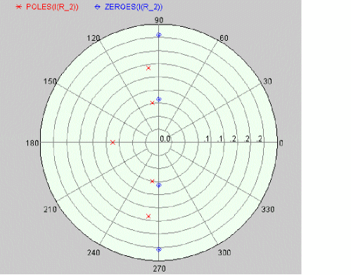Original polar Plot	Filtered polar plot

r2d (radians-to-degrees)

Converts a scalar or waveform expressed in radians to degrees.

Syntax

r2d( arg )

r2d( arg=arg )

Arguments

arg

The signal.

Example

export real myr2d = r2d( 3.14 )

returns

myr2d = 179.909

re

Returns the real portion of a complex number.

Syntax

re( arg )

re( arg=arg )7

Arguments

arg

The complex number.

Examples

export real myre = re( cplx(1,2) )

returns

myre = 1

export real real_sll = re( s(1,1) )

returns

real_sll = 0.682203

real

Creates a real number from an integer number.

Syntax

real( arg )

real( arg=arg )

Arguments

arg

The integer.

risetime

Returns the rise time for a signal measured between percent low and percent high of the difference between the initial and final value.

You can use the risetimes function to obtain the rise time for all edges instead of a single edge returned by the risetime function.

Syntax

risetime( sig[, initval[, finalval [, inittype[, finaltype[, theta1[, theta2[, xtol[, ytol[, accuracy]]]]]]]]] )

risetime( sig=sig, initval=initval, finalval=finalval [, inittype=inittype] [, finaltype=finaltype] [, theta1=theta1] [, theta2=theta2] [, xtol=xtol] [, ytol=ytol] [, accuracy=accuracy] )

Arguments

sig	The signal.
initval	The X value (if inittype is `’x`) or Y value (if inittype is `’y`) that starts the rise time interval. The measurement is always done in ordinate values.
finalval	The X value (if inittype is `’x`) or Y value (if inittype is `’y`) that ends the rise time interval.
inittype	When `’x`, the initial value is an X value. When `’y`, the initial value is a Y value. Valid values: `’x, ’y` Default: `’y`
finaltype	When `’x`, the final value is an X value. When `’y`, the final value is a Y value. Valid values: `’x, ’y` Default: `’y`
theta1	The percent low. Default: `10`
theta2	The percent high. Default: `90`
xtol	The relative tolerance in percentage value in the X direction. Default: `1`
ytol	The relative tolerance in percentage value in the Y direction. Default: `1`
accuracy	Specifies whether the function should use interpolation, or use iteration controlled by the absolute tolerances to calculate the value. `’interp` directs the function to use interpolation, and `’exact` directs the function to consider the xtol and yval values. Data types: name for scalar Valid values: `’interp`, `’exact` Default: `’exact`

Example 1

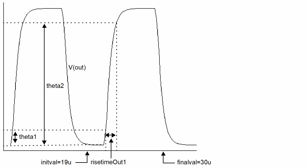
export real risetimeOut1 = risetime( sig=V(out), initval=19u, finalval=30u, inittype=’x, finaltype=’x, theta1=10, theta2=90)

The following diagram illustrates how the result from the above example is determined.

Example 2

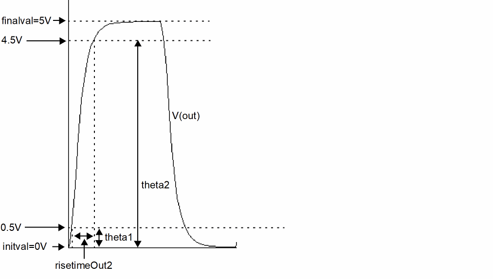
export real risetimeOut2 = risetime( sig=V(out), initval=0V, finalval=5V, inittype=’y, finaltype=’y, theta1=10, theta2=90)

The following diagram illustrates how the result from the above example is determined.

rmsnoise

Returns the root mean square noise of a signal. The root mean square is defined as:

rmsnoise=sqrt{ integral[Sig(t) * Sig(t)] }

Syntax

rmsnoise( sig:param )

rmsnoise( sig=sig:param )

Arguments

sig	The signal.
param	The parameter that refers to the noise to be provided. Possible values are `out` (output noise), `in` (input noise), `F` (noise factor), `NF` (noise figure) and `gain` (circuit gain).

Example

export real total_noise = rmsnoise ( myNoise:out )

SpectreMDL returns the total output referred noise from the pre-defined noise analysis myNoise.

rms (root-mean-square)

Returns the root mean square of a signal.

Syntax

rms( sig )

rms( sig=sig )

Arguments

sig

The signal.

Example

export real rmsOut = rms( V(out))

round

Rounds a number to the closest integer value.

Syntax

round( arg )

round( arg=arg )

Arguments

arg

The number.

Example

export real myround = round( 1.234 )

returns

myround = 1

S

Returns the complex value of Scattering (S) parameter of a network. Only available from sp analysis results.

Syntax

s( rowindex, colindex )

s(rowIndex=rowIndex, colIndex=colIndex )

Arguments

rowindex	The scattering matrix row index.
colindex	The scattering matrix column index.

In general, the 2-port network S-parameter definitions are:

s(1,1) input port voltage reflection coefficient

s(1,2) reverse voltage gain

s(2,1) forward voltage gain

s(2,2) output port voltage reflection coefficient

If used with the functions like db, angle, re or im, the real number value is returned:

db(s(1,1)) returns the db of s(1,1)

angle(s(1,1)) returns the phase of s(1,1) in degrees

ph(s(1,1)) returns the phase of s(1,1) in radians

re(s(1,1)) returns the real part of s(1,1)

im(s(1,1)) returns the image part of s(1,1)

Example

export real ft = cross( sig = ( db(s(2,1) ) ), dir = ’cross, n=1 )

returns

ft = 3.68369e+09

sample

Returns a waveform or an array representing a sample of the signal based on step size or points per decade.

Syntax

sample( sig, from, to, by, type )

sample( sig=sig, from=from, to=to, by=by, type=type )

Arguments

sig	The signal.
from	The X-axis value at which the sampling begins.
to	The X-axis value at which the sampling stops.
type	Specifies whether the sample should be linear or logarithmic. Valid values: `’linear`, `’log` Default value: `’linear`
by	If type is `’linear`, specifies the step size for the sample. If type is `’log`, specifies the points per decade.

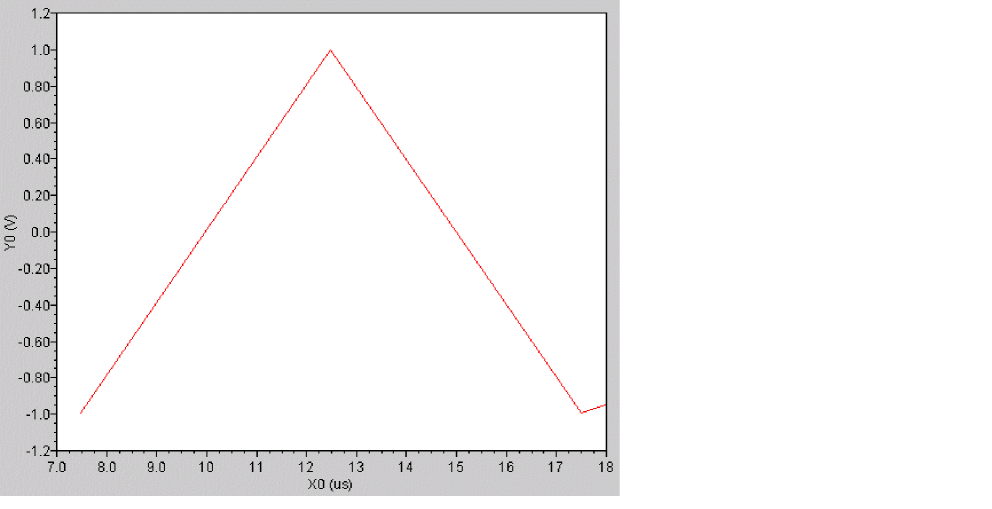
Example 1

export real sampleOut = sample(sig=V(2), from=7.5us, to=18us, by=5us, type=’linear)

transforms the following input signal

into the following output signal

Example 2

export real v2smpl[] = sample(sig=V(2), from=10n, to=40n, by=0.1n)

The above example samples signal V(2) into an array as shown below:

v2smp1[0] = 1.08957e-10

v2smp1[1] = 1.21644e-08

v2smp1[2] = 1.8

v2smp1[3] = 2.39729e-07

v2smp1[4] = 1.8

...

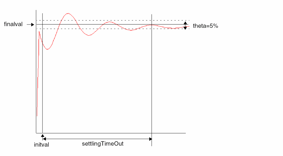
settlingtime

Calculates the time required by a signal to settle at a final value within a specified limit.

Syntax

settlingtime( sig, initval, finalval, inittype, finaltype, theta)

settlingtime( sig=sig, initval=initval, finalval=finalval, inittype=inittype, finaltype=finaltype, theta=theta )

Arguments

sig	The signal.
initval	The starting value for the measurement.
finalval	The final value for the measurement.
inittype	Specifies whether initval is an X-axis or Y-axis value. If it is `’x`, initval is the X-axis value. If it is `’y`, initval is the Y-axis value.
finaltype	Specifies whether finalval is an X-axis or Y-axis value. If it is `’x`, finalval is the X-axis value. If it is `’y`, finalval is the Y-axis value and the signal settles at finalval until the end.
theta	Percentage of (finalval-initval) within which the signal has to settle.

Example

export real settlingTimeOut = settlingtime( sig=V(out), initval=0, finalval=1.0, inittype=’y, finaltype=’x, theta=5 )

returns

settlingTimeOut = 3.7185180980334184E-5sec

The following diagram illustrates how the result from the above example is determined.

sign

Returns a value that corresponds to the sign of a number.

Syntax

sign( arg )

sign( arg=arg )

Arguments

arg

The number whose sign is to be returned. If the number is greater than zero, the sign function returns 1.0; if the number is equal to zero, the sign function returns 0.0; if the number is less than zero, the sign function returns -1.0.

Example

sign( -17.3)

returns

-1.0

sin

Returns the sine of a signal.

Syntax

sin( arg )

sin( arg=arg )

Arguments

arg

The signal.

Example

export real mysin = sin( 1 )

returns

mysin = 0.84

sinh

Returns the hyperbolic sine of a signal.

Syntax

sinh( arg )

sinh( arg=arg )

Arguments

arg

The signal.

Example

export real mysinh = sinh( 1 )

returns

mysinh = 1.18

size

Returns the size of an array or the number of points in a waveform.

Syntax

size( arg, [, from [, to ] ])

size( arg=arg [, from=from] [, to=to])

Arguments

arg	The signal or the array.
from	The starting abscissa.
to	The ending abscissa

Example 1

run tran(  step=1e-09, pstep=1e-09, stop=9e-02 )

export real signalNum = size( V(R1), 8.9e-022, 9e-02)

returns

signalNum = 108018

Example 2

export real cro = crosses(sig=(V(R1))-(1/ 2),dir='cross,n=int(1))

export real num = size(cro)

returns

cro[0]          =  8.33333e-07

cro[1]          =  4.16583e-06

cro[2]          =  1.08334e-05

cro[3]          =  1.41666e-05

num             = 4

Example 3

export real arr [] = {1.1, 2.2}

export real num = size(arr)

returns

arr[0]    = 1.1

arr[1]    = 2.2

num      = 2

slewrate

Computes the average rate at which the buffer expression changes from percent low to percent high of the difference between the initial value and the final value.

Syntax

slewrate( sig[, initval[, finalval [, inittype[, finaltype[, theta1[, theta2[, xtol[, ytol[, accuracy]]]]]]]]] )

slewrate( sig=sig, initval=initval, finalval=finalval [, inittype=inittype] [, finaltype=finaltype] [, theta1=theta1] [, theta2=theta2] [, xtol=xtol] [, ytol=ytol] [, accuracy=accuracy] )

Arguments

sig	The signal.
initval	The X value (if inittype is `’x`) or Y value (if inittype is `’y`) that starts the rise time interval.
finalval	The X value (if inittype is `’x`) or Y value (if inittype is `’y`) that ends the rise time interval.
inittype	When `’x`, the initial value is an X value When `’y`, the initial value is a Y value. Valid values: `’x, ’y` Default: `’y`
finaltype	When `’x`, the final value is an X value. When `’y`, the final value is a Y value. Default: `’y`
theta1	The percent low. Default: `10`
theta2	The percent high. Default: `90`
xtol	The relative tolerance in percentage value in the X direction. Default: `1`
ytol	The relative tolerance in percentage value in the Y direction. Default: `1`
accuracy	Specifies whether the function should use interpolation, or use iteration controlled by the absolute tolerances to calculate the value. `’interp` directs the function to use interpolation, and `’exact` directs the function to consider the xtol and yval values. Data types: name for scalar Valid values: `’interp`, `’exact` Default: `’exact`

Example

A statement like

export real slewrate1 = slewrate( V(out), 20ns, 60ns )

produces a result similar to

6.337662406448401E7V/s

slice

Returns the slice of an array.

Syntax

slice( arg, from, to, step )

slice( arg=arg, from= from, to = to, step =step)

Arguments

`array`	A user-defined array, or an array that comes from the built-in function.
`from`	Array starting subscript.
`to`	Array ending subscript.
`step`	Array step.

Example

real arr[]={1.0,2.0,3.0,4.0,5.0,6.0,7.0}

export real myslice1=slice(arr,from=2,to=5,step=1)

export real myslice2=slice(arr,from=2,to=5,step=2)

returns

myslice1[0]   =  2

myslice1[1]   =  3

myslice1[2]   =  4

myslice1[3]   =  5

myslice2[0]   =  2

myslice2[1]   =  4

snr

Calculates the signal to noise ratio from a complex frequency based signal.

Syntax

snr( sig, sig_from, sig_to, noise_from, noise_to )

snr( sig=sig, sig_from=sig_from, sig_to=sig_to, noise_from=noise_from, noise_to=noise_to )

Arguments

sig	The signal.
sig_from	The left window border of the signal. The sig_from value must be greater than or equal to noise_from.
sig_to	The right window border of the signal. The sig_to value must be less than or equal to noise_to.
noise_from	The left window border of the noise.
noise_to	The right window border of the noise.

Example

You have the following frequency plot.

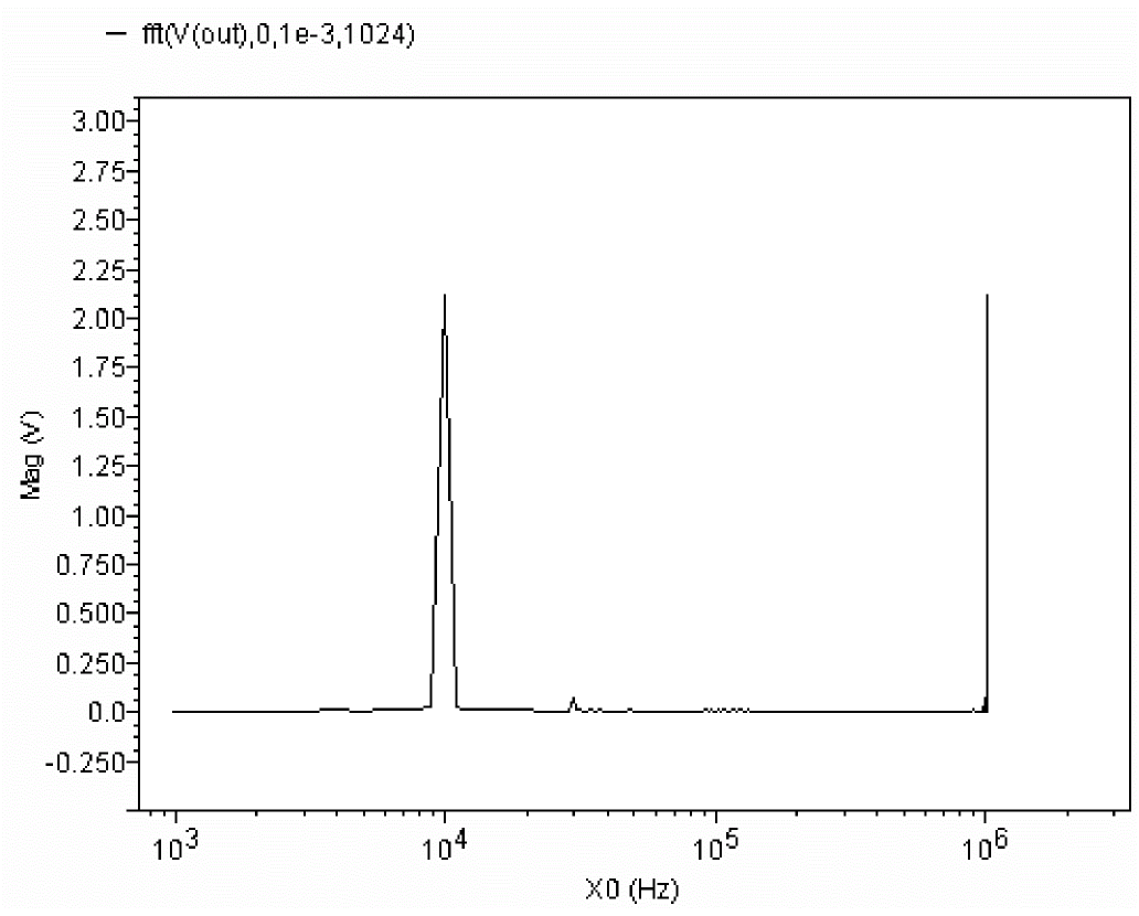
To determine the signal-to-noise ratio, you use the statement

export real snr(fft(V(out),0,1e-3,1024),9e3,11e3,1,500e3)

which, in this case, returns

29.268026738835342dB

spectrumMeas

Calculates Signal-to-Noise-and-Distortion Ratio (SINAD), Spurious Free Dynamic Range (SFDR), Effective Number of Bits (ENOB), and Signal-to-Noise Ratio (without distortion) by using discrete Fourier transform of the clipped portion of any given input signal.

The spectrum measure is used for characterizing A-to-D converters and is typically supported for transient simulation data.

Syntax

spectrumMeas( signal, startTime, endTime, numberofSamples, numberofNoisebins, startFrequency, endFrequency, windowType )

spectrumMeas( signal=signal, startTime=startTime, endTime=endTime, numberofSamples=numberofSamples, numberofNoisebins=numberofNoisebins, startFrequency=startFrequency, endFrequency=endFrequency, windowType=windowType adcspan=adcspan measureType=measureType )

Arguments

signal	The signal to be measured.
startTime	The time to start clipping the signal in the time domain.
numberofSamples	Number of noise bins where the size of one bin is the reciprocal of the data window width. For example, 1 ms of transient data creates a bin size of 1 kHz. Valid values: Any integer power of two greater than or equal to zero. Default value: 0, which implies that no signal is spilling into the bins. A frequency band of bin-size times the number of bins is calculated and adjusted as a function of the selected window. Frequency components in each band to the left and right of the fundamental or the harmonics are set to zero and do not contribute to any output result.
startFrequency	Lower limit of frequency range for the spectrum measures. Default value: First frequency point of the FFT.
endFrequency	Upper limit of frequency range for the spectrum measures. Default value: Last frequency point of the FFT.
windowType	Windowing function applied to the input waveform. Valid values: 0: Rectangular, 1: Blackman, 2: BlackmanHarris, 3: Cosine2, 4: Cosine4, 5: ExtCosBell, 6: HalfCycleSine, 7: HalfCycleSine3, 8: HalfCycleSine6, 9: Hanning, 10: Hamming, 11: Parzen, and 12: Triangular. Default value: 0: Rectangular.
adcSpan	Full-scale span ignoring any DC offsets. This is used in ENOB calculation. Valid values: Any floating point value. Default value: If ADC Span is not specified or is nil, it is assumed to be 0 and is taken to be the peak-to-peak value of the fundamental.
measureType	Result specifier. Valid values: 0:sinad, 1:snhr, 2:sfdr(db), and 3:enob. Default value: 0:sinad."

Example (netlist)

.tran 1n 1000n

.measure tran sinad param=spectrumMeas(V(1), 10ns, 110ns, 200, 0, 0, 0, 0, 0, 0)

.measure tran snhr param=spectrumMeas(V(1), 10ns, 110ns, 200, 0, 0, 0, 0, 0, 1)

.measure tran sfdr param=spectrumMeas(V(1), 10ns, 110ns, 200, 0, 0, 0, 0, 0, 2)

.measure tran enob param=spectrumMeas(V(1), 10ns, 110ns, 200, 0, 0, 0, 0, 0, 3)

Example (MDL file)

alias measurement transient {

    export real sinad, snhr, sfdr, enob

    export real temper

    temper=temp

    run tran( step=1.0000000000000001e-09, pstep=1e-09, stop=1.0000000000000002e-06 )

    sinad=spectrumMeas( V(1),1e-08 ,1.1e-07 ,200 ,0 ,0 ,0 ,0 ,0 ,0 )

    snhr=spectrumMeas( V(1),1e-08 ,1.1e-07 ,200 ,0 ,0 ,0 ,0 ,0 ,1 )

    sfdr=spectrumMeas( V(1) ,1e-08 ,1.1e-07 ,200 ,0 ,0 ,0 ,0 ,0 ,2 )

    enob=spectrumMeas( V(1),1e-08 ,1.1e-07 ,200 ,0 ,0 ,0 ,0 ,0 ,3 )

 run transient as transient1

sqrt

Returns the square root of a signal.

Syntax

sqrt( arg )

sqrt( arg=arg )

Arguments

arg

The signal.

Example

export real mysqrt = sqrt( 4 )

returns

mysqrt = 2

stathisto

Creates a histogram from a signal.

The stathisto function is available from the calculator. It is not supported within a Spectre MDL control file since it returns a scalar and not a waveform.

Syntax

stathisto( sig [, nbins][, min][, max][, innerswpval] )

stathisto(sig=sig [, nbins=nbins] [, min=min] [, max=max] [, innerswpval=inner swpval])

Arguments

sig	The waveform.
nbins	The number of bins to be created.
min	The value that specifies the smaller end point of the range of values included in the histogram.
max	The value that specifies the larger end point of the range of values included in the histogram.
innerswpval	The inner-most sweep parameter in the dataset. You use this parameter to slice through parametric waveforms to extract the data for the histogram. Default: The first available value of time in the dataset.

Example

Assume that you have the results of running a Monte Carlo analysis on top of a transient analysis, so that the inner-most swept variable is time. Now, for the particular value of time specified by the innerswpval argument specification, the stathisto function creates a histogram by analyzing all the Monte Carlo iterations and extracting from each one the value of the signal at the specified time.

For example, to create a histogram for the time 100ns, you might use the following statement.

stathisto(I(V10\:p),innerswpval=100e-9)

To create a histogram for the time 650ps, you might use the following statement.

stathisto(I(V10\:p),innerswpval=.65e-9)

stddev

Returns the standard deviation of a signal. Standard deviation is defined as follows:

sqrt( variance(N) )

Syntax

stddev( arg )

stddev( arg=arg )

Arguments

arg

The signal.

sum

Returns the sum value of an array.

Syntax

sum( arg )

sum( arg=arg )

Arguments

arg

A user-defined array, or an array that comes from the built-in function.

Example

real arr[ ] = {1.0, 2.0, 3.0}

export real mysum=sum(arr)

returns

mysum=6.0

system

Returns a string, which is the output of command executed by shell.

Syntax

system( command )

system( command=command )

Arguments

command

A user-specified shell command.

Example

string d1=system( "date +\"%y%m%d%H%M\"" );

print fmt("%s", d1) addto="aa.data"

returns

1302130702

The function should only be used at the top-level MDL file, or before the run command in an alias measurement, and not during analysis.

tan

Returns the tangent of a signal.

Syntax

tan( X )

tan( X=X )

Arguments

X	The scalar or signal.

Example

export real mytan = tan( 1 )

returns

mytan = 1.56

tanh

Returns the hyperbolic tangent of a signal.

Syntax

tanh( arg)

tanh( arg=arg )

Arguments

arg

The scalar or signal.

Example

export real mytanh = tanh( 1 )

returns

mytanh = 0.76

thd

Computes the percentage of the total harmonic distortion (THD) of a signal with respect to the fundamental frequency and is expressed as a voltage percentage.

Syntax

thd( signal, from, to, numberofSamples, fundamental )

thd( signal=signal, from=from, to=to, numberofSamples=numberofSamples, fundamental=fundamental )

Arguments

signal	Signal to be measured
from	Start time of the signal frequency
to	Stop time of the signal frequency
numberofSamples	Number of time domain points to be used
fundamental	Fundamental frequency of the signal

Example (netlist)

.tran 1n 1000n

.measure tran thd param='thd(V(1), 10ns, 110ns, 200, 1G)'

Example (MDL file)

alias measurement transient {

    export real thd

    export real temper

    temper=temp

    run tran( step=1.0000000000000001e-09, pstep=1e-09, stop=1.0000000000000002e-06 )

    thd=thd( V(1) ,1e-08 ,1.1e-07 ,200 ,1000000000 )

trim

Returns the portion of a signal between two points along the abscissa.

Syntax

trim( sig[, from[, to]] )

trim( sig=sig [, from=from] [, to=to] )

Arguments

sig

The signal.

Data types: real for scalar

from

The starting abscissa.

Data types: real for scalar

The ending abscissa.

Data types: real for scalar

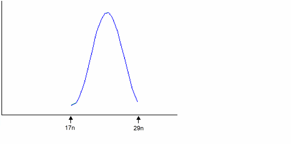
Example 1

The following example works in an MDL control file.

export real trimOut = max ( trim( sig=V(sinewave), from=17n, to=29n ))

In Virtuoso Visualization and Analysis XL,

trim ( sig=V(sinewave), from=17n, to=29n )

transforms the following input signal

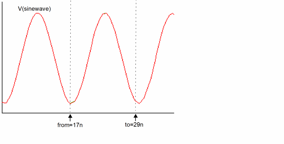
into the following output signal

V

Returns the voltage of a net.

Syntax

V(node)

V(node, node)

V(Instname:term)

V(Instname:term, Instname:term)

V(devname)     //which outputs voltage value between positive and negative terminals of a 2-terminal device.

V(node) takes precedence over V(devname). It is illegal to apply the V probe function to a devname and a node, or a pair of devnames. V can be uppercase or lowercase.

Arguments

node	The net name with or without the hierarchical path.
Instname	The instance name. It can be a N-terminal device instance or a N-terminal subcircuit instance.
devname	The 2-terminal device name (not including the 2-terminal subcircuit instance).
term	The terminal name or terminal index of a device or a subcircuit instance.

Examples

V(p,n)        // Returns the voltage between nodes p and n.

V(Rload:1)    // Returns the voltage from terminal Rload:1 to ground.

V(I0:q)       // Returns the voltage from terminal I0:q to ground.

V(I0:q,I1:y)  //Returns the voltage between terminal I0:q and terminal I1:y.

variance

Returns the statistical variance of a signal. The variance is defined as follows:

1/(N-1) * ( (X1 - mean)^2 + (X2-mean)^2 + .... (XN-mean)^2) ,

where N is the total number of samples.

Syntax

variance( arg)

variance( arg=arg )

Arguments

arg

The scalar or signal.

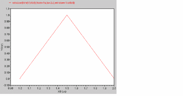
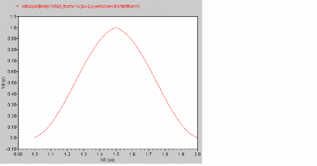
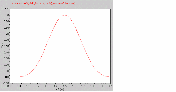
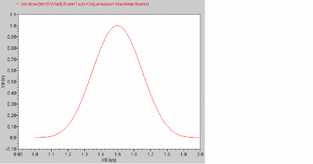
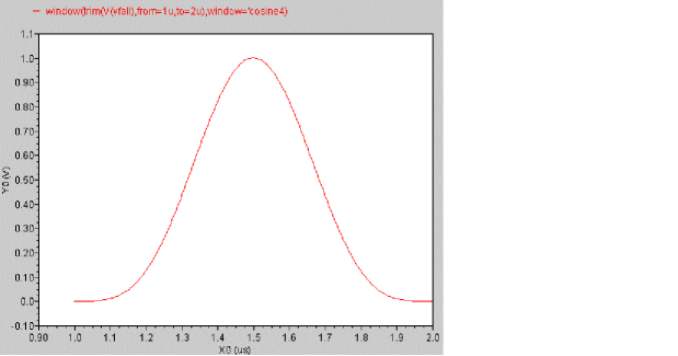
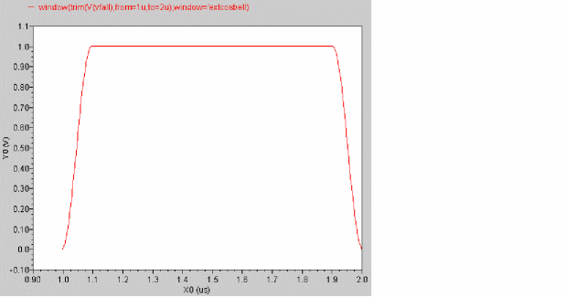
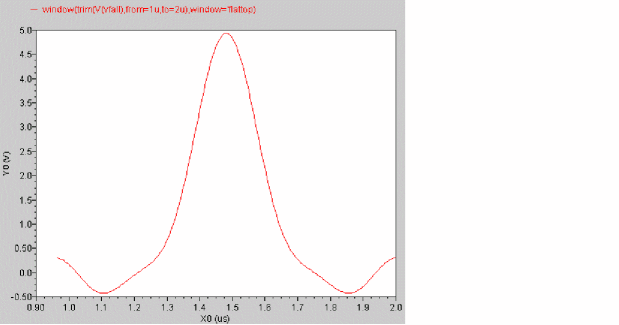
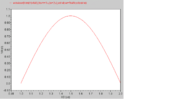
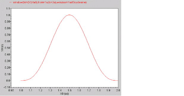
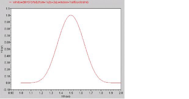
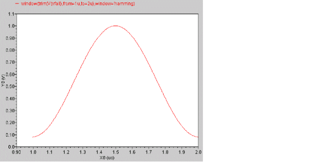
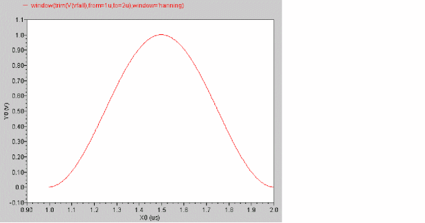
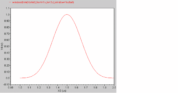
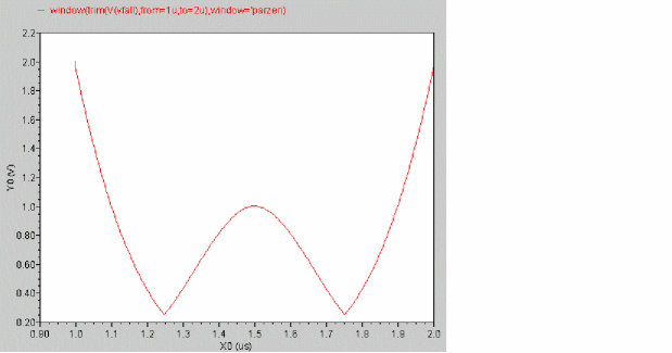
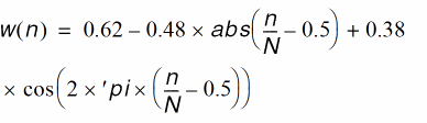
window

Applies the specified window to a signal.

Syntax

window( arg[, window] )

fft( arg=arg[, window=window] )

Arguments

arg

The signal.

window

The window to be applied.

Valid values: ’rectangular, ’bartlett, ’bartletthann, ’blackman, ’blackmanharris,’cosine2, ’cosine4, ’extcosbell, ’flattop, ’halfcyclesine, ’half3cyclesine, ’halfcyclesine3, ’half6cyclesine, ’halfcyclesine6, ’hamming, ’hanning, ’nuttall, ’parzen, ’triangular

Default: ’rectangular

Equations and Examples

This section describes the equations used by each type of window and then shows an example. In the equations:

N = total number of waveform points

n = current waveform point

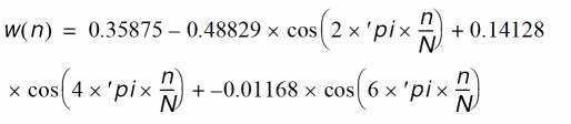
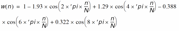
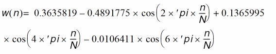
Window	Equation and Example	Where
`’rectangular`
`’bartlett`		0≤n≤N
`’bartlett`		otherwise
`’bartletthann`		0≤n≤N
`’bartletthann`		otherwise
`’blackman`		0≤n≤N
`’blackman`		otherwise
`’blackmanharris`		0≤n≤N
`’blackmanharris`		otherwise
`’cosine2`		0≤n≤N
`’cosine2`		otherwise
`’cosine4`		0≤n≤N
`’cosine4`		otherwise
`’extcosbell`		abs(n/N - 0.5) > 0.4
`’extcosbell`		otherwise
`’flattop`		0≤n≤N
`’flattop`		otherwise
`’halfcyclesine`		0≤n≤N
`’halfcyclesine`		otherwise
`’half3cyclesine` and `’halfcyclesine3`		0≤n≤N
`’half3cyclesine` and `’halfcyclesine3`		otherwise
`’half6cyclesine` and `’halfcyclesine6`		0≤n≤N
`’half6cyclesine` and `’halfcyclesine6`		otherwise
`’hamming`		0≤n≤N
`’hamming`		otherwise
`’hanning`		0≤n≤N
`’hanning`		otherwise
`’nuttall`		0≤n≤N
`’nuttall`		otherwise
`’parzen`		abs(2*n/N-1)≤0.5
`’parzen`		otherwise
`’triangular`	Same as bartlett. For more information, see `’bartlett`.

xval

Returns the vector consisting of the abscissas of the points in the signal.

Syntax

xval( arg )

xval( arg=arg )

Arguments

arg

The signal.

Example 1

export real xvalOut = max ( xval( V(out) ) )

Returns the maximum X-axis value for V(out).

Example 2

export real xvalMax=xval(max(V(out)))

Returns the X-axis value of the point where V(out) is at its maximum voltage value.

Y

Returns the complex value of the Admittance (Y) parameter of a network.

Syntax

y( rowindex, colindex )

y(rowIndex=rowIndex, colIndex=colIndex )

Arguments

rowindex	The admittance matrix row index. The value can be scalar.
colindex	The admittance matrix column index. The value can be scalar.

Example

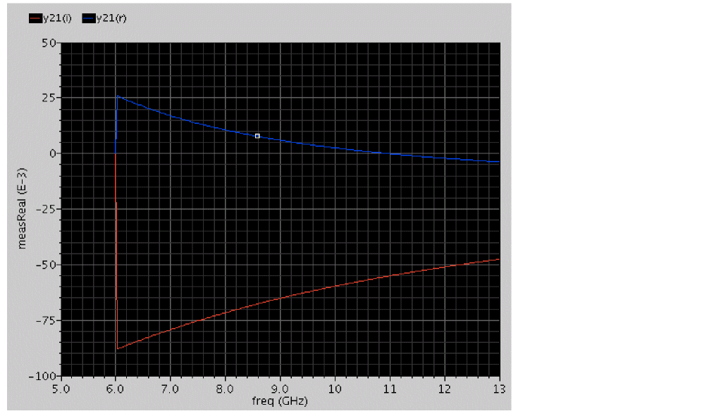
real __mdlvar_13=_hprobe( "y21(r)", re(y(2,1)) )

real __mdlvar_14=_hprobe( "y21(i)", im(y(2,1)) )

The output looks like below.

yval

Returns a vector consisting of the ordinates of the points in the signal. This function can also calculate the ordinate value at a specified abscissa value.

Syntax

yval( arg )

yval( arg=arg )

Arguments

arg

The signal.

Example 1

export real yvalOut = max ( yval( V(out) ) )

Returns the maximum Y-axis value for V(out).

Example 2

export real yvalOut1 = yval ( V(out)@ 100ns )

returns

3.467928474540306

Z

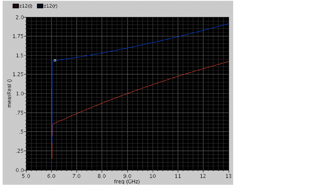
Returns the complex value of Impedance (Z) parameter of a network.

Syntax

z( rowindex, colindex )

z(rowIndex=rowIndex, colIndex=colIndex )

Arguments

rowindex	The impedance matrix row index. The value can be scalar.
colindex	The impedance matrix column index. The value can be scalar.

Example

real __mdlvar_7=_hprobe( "z22(r)", re(z(2,2)) )

real __mdlvar_8=_hprobe( "z22(i)", im(z(2,2)) )

The output looks like below.

Return to top

Spectre Circuit Simulator Measurement Description Language User Guide and ReferenceProduct Version 23.1, June 2023

A

Built-In Functions

abs

Syntax

Arguments

Example

acos

Syntax

Arguments

Example

acosh

Syntax

Arguments

Example

analstop

Syntax

Arguments

Example

angle

Syntax

Arguments

Example 1

Example 2

argmax

Syntax

Arguments

Example

argmin

Syntax

Arguments

Example

asin

Syntax

Arguments

Example

asinh

Syntax

Arguments

Example

atan

Syntax

Arguments

Example

atanh

Syntax

Arguments

avg

Syntax

Arguments

Example

avgdev

Syntax

Arguments

bw (bandwidth)

Syntax

Arguments

Example

ceil

Syntax

Arguments

Example

cfft

Syntax

Arguments

clip

Syntax

Arguments

Example 1

Example 2

conj

Syntax

Arguments

Example

convolve

Syntax

Arguments

Equation

Example

cos

Spectre Circuit Simulator Measurement Description Language User Guide and Reference
Product Version 23.1, June 2023

b w (bandwidth)