2 The Spectre RF Analyses

Spectre^®circuit simulator RF analysis (Spectre RF) provides unique analyses that are useful on RF circuits. These analyses directly compute the steady-state response and the small-signal behavior of circuits that exhibit frequency translation.

The individual Spectre RF analyses described in this section are

PSS (large-signal analysis). See “Periodic Steady-State Analysis (PSS)”.
PAC (small-signal analysis). See “Periodic AC Analysis (PAC)”.
PSP (small-signal analysis). See “Periodic S-Parameter Analysis (PSP)”.
PXF (small-signal analysis). See “Periodic Transfer Function Analysis (PXF)”.
Pnoise (small-signal analysis). See “Periodic Noise Analysis (Pnoise)”.
PSTB (periodic stability analysis). See “Periodic Stability Analysis (PSTB)”.
QPSS (large-signal analysis). See “Quasi-Periodic Steady-State Analysis (QPSS)”.
QPnoise (small-signal analysis). See “Quasi-Periodic Noise Analysis (QPnoise)”.
QPAC (small-signal analysis). See “Quasi-Periodic AC Analysis (QPAC)”.
QPSP (small-signal analysis). See “Quasi-Periodic S-Parameter Analysis (QPSP)”.
QPXF (small-signal analysis). See “Quasi-Periodic Transfer Function Analysis (QPXF)”.
ENVLP (envelope analysis). See “Envelope Analysis (ENVLP)”.
HB (large-signal analysis). See “Harmonic Balance Steady State Analysis (HB)”.
HBAC (small-signal analysis). See “Harmonic Balance AC Analysis (HBAC)”.
HBnoise (small-signal analysis). See “Harmonic Balance Noise Analysis (HBnoise)”.
HB S-Parameter Analysis (hbsp). See “HB S-Parameter Analysis (hbsp)”
Envelope Analysis (ENVLP). See “Envelope Analysis (ENVLP)”

Periodic Steady-State Analysis (PSS)

The PSS analysis computes the periodic steady-state response of a circuit at a specified fundamental frequency, with a simulation time independent of the time-constants of the circuit. The PSS analysis also determines the circuit’s periodic operating point which is the required starting point for the periodic time-varying small-signal analyses: PAC, PSP, PXF, and Pnoise.

The Shooting Method

Spectre RF simulation traditionally uses a technique called the shooting method to implement PSS analysis. This method is an iterative, time-domain method which starts with a guess or estimate of the initial condition and ultimately finds an initial condition that directly results in a steady-state solution.

The shooting method requires few iterations if the final state of the circuit after one period is a near-linear function of the initial state. This is usually true even for circuits that have strongly nonlinear reactions to large stimuli (such as the clock or the local oscillator). Typically, shooting methods need about five iterations on most circuits, and they easily simulate the nonlinear circuit behavior within the shooting interval.

Cadence’s Fourier integral method, a new approach to Fourier analysis, makes PSS analysis using the shooting engine more accurate with strongly nonlinear circuits than previous methods. Cadence’s Fourier integral method approaches the accuracy of harmonic balance simulators for near-linear circuits, and far exceeds it for strongly nonlinear circuits.

In the case of a driven circuit, when you set errpreset to either moderate or conservative, Spectre RF automatically performs a high-order refinement after the shooting method. Spectre RF uses the Multi-Interval Chebyshev polynomial spectral algorithm (MIC) to refine the simulation results. When you set highorder to no, MIC is turned off. However, when you set highorder to yes, Spectre RF tries harder to converge. In a case where MIC fails to converge, Spectre RF falls back to the original PSS solution. For more information, see “The High-Order and Finite Difference Refinement Parameters” and “The errpreset Parameter in PSS Analysis”.

You can also use the finite difference (FD) refinement method after the shooting method to refine the simulation results. For more information, see “The High-Order and Finite Difference Refinement Parameters”.

Parameters for PSS Analysis

For more information on PSS analysis parameters, refer to the Periodic Steady-State Analysis (pss) section in the Spectre Circuit Simulation Reference manual.

The PSS Algorithm for Driven and Autonomous Circuits

The PSS analysis works with both autonomous and driven circuits.

Driven circuits require some time-varying stimulus to generate a time-varying response.
Some common driven circuits include amplifiers, filters, mixers, and so on.
Autonomous circuits are time-invariant circuits with time-varying responses. Thus, autonomous circuits generate non-constant waveforms even though they are not driven by a time-varying stimulus.
The most common autonomous circuit is an oscillator.

See “Autonomous PSS Analysis” for additional information on the algorithm for PSS analysis of autonomous circuits.

The errpreset parameter works differently for autonomous and driven circuits. For detailed information, see “The errpreset Parameter in PSS Analysis”.

Driven PSS Analysis

A PSS analysis using the shooting method consists of two phases

The initial transient phase, a standard transient analysis to initialize the circuit.
The shooting phase, to compute the periodic steady-state solution for the circuit using the shooting method.

The Initial Transient Phase of PSS Analysis

The initial transient analysis provides a flexible mechanism to direct the circuit to a particular steady-state solution you are interested in and to avoid undesired solutions. Another use of the initial transient simulation is to help convergence by eliminating large but fast decaying modes that are present in many circuits. For example, in the case of driven circuits, consider the reset signal in Figure 2-1.

PSS starts by performing a loose transient analysis for the interval from t _start to t _stop where t _stop is t _onset + t _stab + period . This initial loose transient analysis disregards your errpreset setting and performs a transient analyses with errpreset=liberal. If the initial transient results are relevant, you can output them by setting saveinit to yes. The steady-state results are always computed for the specified period, from t _init to t _stop. By default, t _start and t _stab are set to zero, while t _init, t _onset and t _stop are always automatically generated and your errpreset settings are used.

Figure 2-1 Initial Transient Analysis and Timing Relationships for PSS Analysis

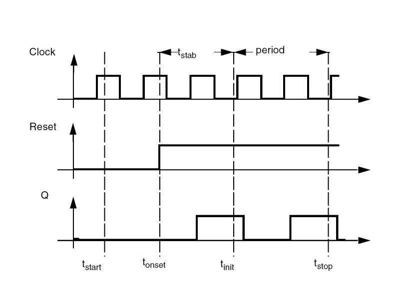
The first interval begins at tstart, which is normally 0, and continues through the onset of periodicity t _onset for the independent sources. The onset of periodicity, which is automatically generated, is the earliest time for which all sources are periodic. The second interval is an optional user specified stabilization interval whose length is tstab. The final interval whose length is period for driven circuits, and estimated as 4x period for autonomous circuits, has a special use for the autonomous PSS analysis—the autonomous PSS analysis monitors the waveforms in the circuit and develops a better estimate of the oscillation period. As is true for transient analysis, the DC solution is the initial condition for the PSS analysis unless you specify otherwise.

Table 2-1 Timing Intervals for PSS Analysis

t start	Start time, `tstart`, for the transient analysis that you specify. This value can be negative or positive and defaults to 0.
t onset	Time when the last stimulus waveform becomes periodic. This value is automatically determined by the simulator for built-in independent sources.
t stab	Additional time that you specify to let the circuit settle. The `tstab` parameter is useful if you want a particular solution for a circuit that has multiple periodic solutions. A long t _stab might also improve convergence.
t init	Time when the PSS analysis begins. tinit = t stab + max (t start , tonset).
period	Analysis interval for the PSS analysis determined from the fundamental frequency (`fund`) or the `period` that you specify.
t stop	Time when the PSS analysis ends. tstop = tinit + period .

The Shooting Phase

After the initial transient phase is complete, the shooting phase begins. During the shooting phase, the circuit is repeatedly simulated over one period while adjusting the initial condition (and the period for autonomous circuits) to find the periodic steady-state solution.

PSS analysis estimates the initial condition for subsequent transient analyses with an interval period . For an accurate estimate for this initial condition, the final state of the circuit must closely match its initial state. PSS then performs a transient analysis, prints the maximum mismatch, and, if the convergence criteria are not satisfied, generates an improved estimate of the necessary initial condition.

This procedure repeats until the simulation converges. Typically, the simulation requires three to five such iterations to reach the steady-state circuit response. After completion, if you request it, PSS computes the frequency-domain response.

In some circuits, the linearity of the relationship between the initial and final states depends on when the shooting interval begins. Theoretically, the starting time of the shooting interval does not matter, as long as it begins after the stimuli become periodic. Practically, it is better to start the shooting interval when signals are quiescent or changing slowly and to avoid starting times when the circuit displays strongly nonlinear behavior. Choosing a poor starting time slows the analysis.

For driven circuits, you can use writepss and readpss to save or reuse the steady state solution from a previously converged PSS simulation.

Within the Analog Circuit Design Environment, you

Define tstart in the SImulation Interval Parameters section of the PSS Options form.
Define tstab in the Additional Time for Stabilization section of the PSS Choosing Analyses form.

The PSS analysis determines the period value from the fundamental frequency (fund) you specify in the Fundamental Tones (PSS and QPSS) section of the PSS Choosing Analyses form.

You can save the initial transient results by setting saveinit to yes. The steady-state results are always computed for the period from t init to t stop . By default, t start (tstart) and t stab (tstab) are set to zero, while t init , t onset , and t stop are always automatically computed.

Use the skipdc Initial-Condition Parameter to specify rampup before the transient (tstab) analysis. Use skipdc only for very special cases where there are several DC solutions in the system.

Set skipdc=no to calculate the initial solution using the usual DC analysis. (This is the default.) Set skipdc=yes to use either the initial solution given in the readic parameter file or the values specified on the ic statements.

When you set skipdc=sigrampup, independent source values start at 0 and ramp up to their initial values during the first phase of the simulation. After the rampup phase, waveform production is enabled in the time-varying independent source.The rampup simulation is from t _start to time=0 seconds. The main simulation is from time=0 seconds to t _stab. If you do not specify the t _start parameter, the default start time is set to -0.1∗ t _stab.

For driven circuits, you specify either the period of the analysis, the period parameter, or its corresponding fundamental frequency, the fund parameter. The period parameter value must be an integer multiple of the period of the drive signals.

Autonomous PSS Analysis

Because autonomous circuits do not have drive signals and you do not know the actual period of oscillation before you run a simulation, you estimate the oscillation period and the PSS analysis computes the precise period along with the periodic solution waveforms. Autonomous circuits, such as oscillators, however, have time-varying responses and generate non-constant waveforms even though the circuits themselves are time-invariant.

PSS analysis of an autonomous circuit, requires you to specify a pair of nodes, p and n. In fact this is how PSS analysis determines whether it is being applied to an autonomous or a driven circuit. If the pair of nodes is supplied, the PSS analysis assumes the circuit is autonomous; if not, the circuit is assumed to be driven. See Spectre Circuit Simulator and Accelerated Parallel Simulator RF Analysis in ADE Explorer User Guide for an example.

Phases of Autonomous PSS Analysis

A PSS analysis has two phases,

A transient analysis phase to initialize the circuit.
A shooting phase to compute the periodic steady state solution.

The transient analysis phase is divided into three intervals:

A beginning interval that starts at tstart, which is normally 0, and continues through the onset of periodicity for the independent sources.
A second, optional stabilization interval of length tstab.
A final interval that is four times the estimated oscillation period specified in the PSS Analysis form. During the final interval, the PSS analysis monitors the waveforms in the circuit and improves the estimate of the oscillation period.

During the first stage of the transient phase, PSS extracts the fundamental frequency from the set of nodes specified in the PSS statement. During the second stage, the PSS analysis examines all the nets in your design to verify the accuracy of the extracted PSS fundamental frequency. This enhancement improves PSS analysis of circuits with frequency dividers by re-evaluating the PSS fundamental to take into account the frequency division in your circuit.

Increasing the tstab Interval

In some cases when an autonomous PSS analysis does not converge after a few iterations, increasing the tstab interval makes convergence faster and easier.

Adjusting the tstab interval might improve the shooting interval starting point by moving it such that signals are quiescent or changing slowly. This allows strongly nonlinear circuits to converge faster.

For oscillator circuits, Spectre RF increases the tstab interval when:

The current Iteration is close to the maximum number of iterations, but the related Norm is still large.

(Iter >= 0.8 * MaxIters && Norm > 1000.0
(Iter >= 0.9 * MaxIters && Norm > 100.0)
(Iter >= 0.95* MaxIters && Norm > 10.0)
(Iter >= MaxIters    && Norm > 1.0)

The PssPeriod has shrunk to zero
```
(PssPeriod < UsrPssPeriod/1.0e3)
```
The initial transient analysis has failed.

When any of these conditions occur, Spectre RF increases the tstab interval as follows.

4.0*PeriodEstimate + PeriodEstimate*DynamicTstabCounter/6.0

where DynamicTstabCounter is an integer from 1 to 6.

During the shooting phase, the circuit is simulated repeatedly over one period. The length of the period and the initial conditions are modified to find the periodic steady state solution.

Simulation Accuracy Parameters

The accuracy of your simulation results depends on your accuracy parameter settings, not on the number of harmonics you request. It is recommended that you adjust the accuracy parameters using the errpreset parameter settings as described in “The errpreset Parameter in PSS Analysis”.

The errpreset parameter works differently for autonomous and driven circuits. For detailed information, see “The errpreset Parameter in PSS Analysis”.

Several parameters determine the accuracy of the PSS analysis.The steadyratio parameter specifies the maximum allowed mismatch between node voltages or current branches from the beginning of the steady-state period to its end. The steadyratio value is multiplied by the lteratio and reltol parameter values to determine the convergence criterion. The reltol and abstol parameters control the accuracy of the discretized equation solution. These parameters determine how well charge is conserved and how accurately steady-state or equilibrium points are computed. You can set the integration error, or the errors in the computation of the circuit dynamics (such as time constants), relative to the reltol and abstol parameters by setting the lteratio parameter.

You can follow the progress of the steady-state iterations because the relative convergence norm is printed in the simulation log file along with the actual mismatch value at the end of each iteration. The iterations continue until the convergence norm value is below one.

Plotting the Current Spectrum

In order to plot the current or power spectrum for a PSS analysis, or for any of the periodic small signal analyses, you must set up the analysis to put the terminal currents into the rawfiles associated with the steady-state results. To do this, choose Outputs - Save All to display the Save Options form where you set currents=selected and useprobes=yes. You also need to use an iprobe component from the analogLib library.

The High-Order and Finite Difference Refinement Parameters

The highorder parameter specifies the use of the high-order Chebyshev refinement method (MIC) which is used after the shooting method to refine the shooting method’s steady-state solution. The highorder parameter applies only to the driven case and when errpreset is set to either moderate or conservative.

When highorder=no, the MIC method is turned off. This is the default.
When highorder=yes, the MIC method tries harder to converge.
When errpreset is set to either moderate or conservative and highorder is not set by the user, MIC is used but it does not aggressively try to converge unless highorder is explicitly set to yes.

The finitediff parameter specifies the use of the finite difference (FD) refinement method which is used after the shooting method to refine the simulation results. This flag is only meaningful when the highorder flag is set to no.

When finitediff=no, the FD method is turned off.
When finitediff=yes, PSS applies the FD refinement method.
When finitediff=refine, PSS applies the FD refinement method and tries to refine the time steps.

When the simulation uses the 2nd-order method, uniform 2nd order gear is used. When readpss and writepss are used to re-use PSS results, the finitediff parameter automatically changes from no to yes.

Usually FD will eliminate the above mismatch in node voltages or current branches. It can also refine the grid of time steps. In some cases, the numerical error of the linear solver still introduces a mismatch. In this case, you can adjust the steadyratio parameter to a smaller value to activate a tighter tolerance for the iterative linear solver.

The maxacfreq parameter automatically adjusts maxstep to reduce errors due to aliasing in subsequent periodic small-signal analyses. By default, maxacfreq is four times the frequency of the largest harmonic you request, but it is never less than 40 times the fundamental.

The relref parameter determines how the relative error is treated. Table Table 2-2 lists the relref parameter options.

Table 2-2 The relref Parameter Options

Option	Definition
`relref=pointlocal`	Compares the relative errors in quantities at each node to that node alone.
`relref=alllocal`	Compares the relative errors at each node to the largest values found for that node alone for all past time.
`relref=sigglobal`	Compares relative errors in each of the circuit signals to the maximum for all signals at any previous point in time.
`relref=allglobal`	Same as `relref=sigglobal` except that it also compares the residues (KCL error) for each node to the maximum of that node’s past history.

The errpreset Parameter in PSS Analysis

In most cases, errpreset should be the only accuracy parameter you need to adjust. The errpreset parameter quickly adjusts several simulator parameters to fit your needs.

The errpreset parameter works differently for autonomous and driven circuits. For more information see,

Using the errpreset Parameter With Driven Circuits

If your driven (non-autonomous) circuit includes only one periodic tone and you are only interested in obtaining the periodic operating point, set errpreset to liberal. The liberal setting produces reasonably accurate results with the fastest simulation speed. If your driven circuit contains more than one periodic tone and you are interested in intermodulation results, set errpreset to moderate. The moderate setting produces very accurate results. If you want an extremely low noise floor in your simulation results and accuracy is your main interest, set errpreset to conservative.

For both moderate and conservative settings, the Multi-Interval Chebyshev (MIC) algorithm is activated automatically unless you explicitly set highorder=no. If MIC has difficulty converging, the simulator reverts back to the original method. If you set highorder=yes, MIC will continue to attempt to converge.

Table 2-3 shows the effect of the errpreset settings (liberal, moderate, and conservative) on the values of the other parameters used with driven circuits.

Table 2-3 Default Values and Noise Floor for `errpreset` in Driven Circuits

errpreset	reltol	relref	method	Iteratio	steadyratio	maxstep
`liberal`	1e^-3	sigglobal	traponly	3.5	0.001	period/50
`moderate`	1e^-3	alllocal	gear2only	3.5	0.001	period/200
`conservative`1	1e^-4	alllocal	gear2only	*	0.01	period/200

Several parameters determine the accuracy of the PSS analysis. Reltol and abstol control the accuracy of the discretized equation solution. These parameters determine how well charge is conserved and how accurately steady-state or equilibrium points are computed.The integration error, or the errors in the computation of the circuit dynamics (such as time constants) relative to reltol and abstol are set by the lteratio parameter.

These errpreset settings include a default reltol value which is an enforced upper limit for reltol. The only way to decrease the reltol value is with the options statement. The only way to relax the reltol value is to change the errpreset setting.

For a weakly nonlinear circuit, the estimated numerical noise floor is -70 dB for liberal, -90 dB for moderate, and -120 dB for conservative errpreset settings. For a linear circuit, the noise floor is even lower. Multi-interval Chebyshev (MIC) is activated when you explicitly set highorder=yes, which drops the numerical noise floor by at least 30 dB. MIC falls back to the original method if it encounters difficulty converging. You can tighten the psaratio to further drop the numerical noise floor. Spectre RF sets the value of maxstep so that it cannot be larger than the value given in Table 2-3. Except for the reltol and maxstep parameters, errpreset does not change the value of any parameters you have explicitly set. The actual values used for the PSS analysis are given in the log file. If errpreset is not specified in the netlist, liberal settings are used.

Using the errpreset Parameter With Autonomous Circuits

For an autonomous circuit, if you want a fast simulation with reasonable accuracy, set errpreset to liberal. For greater accuracy, set errpreset to moderate. For greatest accuracy, set errpreset to conservative.

Table 2-4 shows the effect of the errpreset settings (liberal, moderate, and conservative) on the values of parameters used with autonomous circuits.

Table 2-4 Default Values and maxstep for `errpreset` in Autonomous Circuits

errpreset	reltol	relref	method	Iteratio	steadyratio	maxstep
`liberal`	1e^-3	sigglobal	traponly	3.5	0.001	period/50
`moderate`	1e^-4	alllocal	gear2only	3.5	0.01	period/200
`conservative`2	1e^-5	alllocal	gear2only	*	0.1	period/400

These errpreset settings include a default reltol value which is an enforced upper limit for reltol. The only way to decrease the reltol value is in the options statement. The only way to increase the reltol value is to change the errpreset setting. Spectre RF sets the maxstep parameter value so that it is no larger than the value given in Table 2-4. Except for the reltol and maxstep values, the errpreset setting does not change any parameter values you have explicitly set. The actual values used for the PSS analysis are given in the log file.

The value of reltol can be decreased from the default value in the options statement. The only way to increase reltol is to relax errpreset. Spectre RF sets the value of maxstep so that it cannot be larger than the value given in Table 2-4. Except for reltol and maxstep, errpreset does not change the value of any parameters you have explicitly set. The actual values used for the PSS analysis are given in the log file. If errpreset is not specified in the netlist, liberal settings will be used. Multi-interval Chebyshev (MIC) is activated when you explicitly set highorder=yes, which will drop the numerical noise floor by at least 30 dB. MIC falls back to the original method if it encounters difficulty converging. You can tighten psaratio to further drop the numerical noise floor.

Other Parameters

A long stabilization (by specifying a large tstab) can help with the PSS convergence. However it can slow down simulation. By default, in the stabilization stage, reltol=1e-3; maxstep=period/25; relref=sigglobal; and method=traponly. They are overwritten when maxstep, relref, or tstabmethod are specified explicitly in pss statement, or reltol is specified explicitly in options statement.

If the circuit you are simulating can have infinitely fast transitions (for example, a circuit that contains nodes with no capacitance), Spectre RF might have convergence problems. To avoid this, you must prevent the circuit from responding instantaneously. You can accomplish this by setting cmin, the minimum capacitance to ground at each node, to a physically reasonable nonzero value. This often significantly improves convergence.

You may specify the initial condition for the transient analysis by using the ic statement or the ic parameter on the capacitors and inductors. If you do not specify the initial condition, the DC solution is used as the initial condition. The ic parameter on the transient analysis controls the interaction of various methods of setting the initial conditions. The effects of individual settings are

`ic=dc`	Any initial condition specifiers are ignored, and the DC solution is used.
`ic=node`	The `ic` statements are used, and the `ic` parameter on the capacitors and inductors are ignored.
`ic=dev`	The `ic` parameters on the capacitors and inductors are used, and the `ic` statements are ignored.
`ic=all`	Both the `ic` statements and the `ic` parameters are used, and the `ic` parameters override the `ic` statements.

If you specify an initial condition file with the readic parameter, initial conditions from the file are used, and any ic statements are ignored.

After you specify the initial conditions, Spectre RF computes the actual initial state of the circuit by performing a DC analysis. During this analysis, Spectre RF forces the initial conditions on nodes by using a voltage source in series with a resistor whose resistance is rforce (see options).

With the ic statement it is possible to specify an inconsistent initial condition (one that cannot be sustained by the reactive elements). Examples of inconsistent initial conditions include setting the voltage on a node with no path of capacitors to ground or setting the current through a branch that is not an inductor. If you initialize Spectre RF inconsistently, its solution jumps; that is, it changes instantly at the beginning of the simulation interval. You should avoid such changes if possible because Spectre RF can have convergence problems while trying to make the jump.

You can skip the DC analysis entirely by using the parameter skipdc. If the DC analysis is skipped, the initial solution will be either trivial, or given in the file you specified by the readic parameter, or, if the readic parameter is not given, the values specified on the ic statements. Device-based initial conditions are not used for skipdc. Nodes that you do not specify with the ic file or ic statements will start at zero. You should not use this parameter unless you are generating a nodeset file for circuits that have trouble in the DC solution; it usually takes longer to follow the initial transient spikes that occur when the DC analysis is skipped than it takes to find the real DC solution. The skipdc parameter might also cause convergence problems in the transient analysis.

The possible settings of parameter skipdc and their meanings are

skipdc=no

Initial solution is calculated using the normal DC analysis (default).

skipdc=yes

Initial solution is given in the file specified by the readic parameter or the values specified on the ic statements.

skipdc=sigrampup

Independent source values start at 0 and ramp up to their initial values in the first phase of the simulation. The waveform production in the time-varying independent source is enabled after the rampup phase.

The rampup simulation is from tstart to time=0 s, and the main simulation is from time=0 s to tstab.
If the tstart parameter is not specified, the default tstart time is set to -0.1*tstab.

Nodesets help find the DC or initial transient solution. You can supply them in the circuit description file with nodeset statements, or in a separate file using the readns parameter. When nodesets are given, Spectre RF computes an initial guess of the solution by performing a DC analysis while forcing the specified values onto nodes by using a voltage source in series with a resistor whose resistance is rforce. Spectre RF then removes these voltage sources and resistors and computes the true solution from this initial guess.

Nodesets have two important uses. First, if a circuit has two or more solutions, nodesets can bias the simulator towards computing the desired one. Second, they are a convergence aid. By estimating the solution of the largest possible number of nodes, you might be able to eliminate a convergence problem or dramatically speed convergence.

When you simulate the same circuit many times, we suggest that you use both the write and readns parameters and give the same file name to both parameters. The DC analysis then converges quickly even if the circuit has changed somewhat since the last simulation, and the nodeset file is automatically updated.

Nodesets and initial conditions have similar implementation but produce different effects. Initial conditions actually define the solution, whereas nodesets only influence it. When you simulate a circuit with a transient analysis, Spectre RF forms and solves a set of differential equations. However, differential equations have an infinite number of solutions, and a complete set of initial conditions must be specified in order to identify the desired solution. Any initial conditions you do not specify are computed by the simulator to be consistent. The transient waveforms then start from initial conditions. Nodesets are usually used as a convergence aid and do not affect the final results. However, in a circuit with more than one solution, such as a latch, nodesets bias the simulator towards finding the solution closest to the nodeset values.

The method parameter specifies the integration method. The possible settings and their meanings are

`method=euler`	Backward-Euler is used exclusively.
`method=traponly`	Trapezoidal rule is used almost exclusively.
`method=trap`	Backward-Euler and the trapezoidal rule are used.
`method=gear2only`	Gears second-order backward-difference method is used almost exclusively.
`method=gear2`	Backward-Euler and second-order Gear are used.

The trapezoidal rule is usually the most efficient when you want high accuracy. This method can exhibit point-to-point ringing, but you can control this by tightening the error tolerances. For this reason, though, if you choose very loose tolerances to get a quick answer, either backward-Euler or second-order Gear will probably give better results than the trapezoidal rule. Second-order Gear and backward-Euler can make systems appear more stable than they really are. This effect is less pronounced with second-order Gear or when you request high accuracy.

Spectre RF provides two methods for reducing the number of output data points saved: strobing, based on the simulation time, and skipping time points, which saves only every Nth point.

The parameters strobeperiod and strobedelay control the strobing method. strobeperiod sets the interval between points that you want to save, and strobedelay sets the offset within the period relative to skipstart. The simulator forces a time step on each point to be saved, so the data is computed, not interpolated.

The skipping method is controlled by skipcount. If this is set to N, then only every Nth point is saved.

The parameters skipstart and skipstop apply to both data reduction methods. Before skipstart and after skipstop, Spectre RF saves all computed data.

The default value for compression is no. The output file stores data for every signal at every time point for which Spectre RF calculates a solution. Spectre RF saves the x axis data only once, because every signal has the same x value. If compression=yes, Spectre RF writes data to the output file only if the signal value changes by at least 2*the convergence criteria. In order to save data for each signal independently, x axis information corresponding to each signal must be saved. If the signals stay at constant values for large periods of the simulation time, setting compression=yes results in a smaller output data file. If the signals in your circuit move around a lot, setting compression=yes results in a larger output data file.

Periodic AC Analysis (PAC)

The Periodic AC (PAC) small-signal analysis computes transfer functions for circuits that exhibit frequency translation. Such circuits include mixers, switched-capacitor filters, samplers, lower noise amplifier, sample-and-holds, and similar circuits. A PAC analysis cannot be used alone. It must follow a large signal PSS analysis. However, any number of periodic small-signal analyses, such as PAC, PSP, PXF, PNoise, can follow a PSS analysis.

PAC analysis is a small-signal analysis like AC analysis, except the circuit is first linearized about a periodically varying operating point as opposed to a simple DC operating point. Linearizing about a periodically time-varying operating point allows transfer-functions that include frequency translation, whereas simply linearizing about a DC operating point could not because linear time-invariant circuits do not exhibit frequency translation. Also, the frequency of the sinusoidal stimulus is not constrained by the period of the large periodic solution.

Computing the small-signal response of a periodically varying circuit is a two step process. First, the small stimulus is ignored and the periodic steady-state response of the circuit to possibly large periodic stimulus is computed using PSS analysis. As a normal part of the PSS analysis, the periodically time-varying representation of the circuit is computed and saved for later use. The second step is applying the small stimulus to the periodically varying linear representation to compute the small signal response. This is done using the PAC analysis.

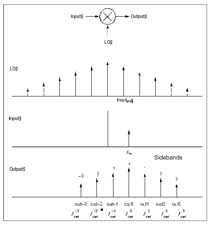
When you apply a small sinusoid to a linear time-invariant circuit, the steady-state response is a sinusoid at the same frequency. However, when you apply a small sinusoid to a linear circuit that is periodically time-varying, the circuit responds with sinusoids at many frequencies, as is shown in Figure 2-2.

Because PAC is a small-signal analysis, the magnitude and phase of each tone computed by PAC is linearly related to the magnitude and phase of the input signal. PAC computes a series of transfer functions, one for each frequency. These transfer functions are unique because the input and output frequencies are offset by the harmonics of the LO.

The Spectre RF simulation labels the transfer functions with the offsets from the input signal in multiples of the LO fundamental frequency. These same labels identify the corresponding sidebands of the output signals. The labels are used as follows

Label	Definition
`0`	For circuits in which the input and output are at the same frequency, such as switched-capacitor filters, the transfer function or sideband is labeled 0.
`-1`	For down-conversion mixers, the transfer function or sideband is labeled -1 because the output frequency is offset from the input frequency by -1 times the LO frequency.
`+1`	For up-conversion mixers, the transfer function or sideband is labeled +1.
	For samplers, sidebands far from zero might be used.

In Figure 2-2, all transfer functions from -3 to +3 are computed. As shown in the figure, the input signal is replicated and translated by each harmonic of the LO. In down-conversion mixers, the -1 sideband usually represents the IF output.

Figure 2-2 The Small-Signal Response of a Mixer as Computed by PAC Analysis

PAC performance is not reduced if the input and LO frequencies are close or equal.

Unlike other analyses in Spectre RF, the PAC analysis can only sweep frequency.

PAC Synopsis

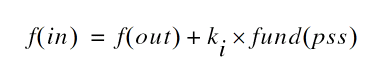
You select the periodic small-signal output frequencies you want by specifying either the maximum sideband (the maxsideband parameter) or an array of sidebands (the sidebands parameter).

For a set of n integer numbers representing the sidebands

the output signal frequency at each sideband is computed as

where

f(in) is the (possibly swept) input frequency
fund(pss) is the fundamental frequency used in the corresponding PSS analysis

If you specify the maximum sideband value as k_max, all 2 × k_max + 1 sidebands from -k_max to +k_max are generated.

The number of requested sidebands does not substantially change the simulation time. However, the maxacfreq of the corresponding PSS analysis should be set to guarantee that | max{f(out)} | is less than maxacfreq, otherwise the computed solution might be contaminated by aliasing effects. The PAC simulation is not executed for |f(in)| greater than maxacfreq. Diagnostic messages are printed for those extreme cases that indicate how to set maxacfreq in the PSS analysis. In the majority of simulations, however, this is not an issue because maxacfreq is never allowed to be smaller than 40x the PSS fundamental.

Intermodulation Distortion Computation

A PSS analysis followed by a PAC analysis measures the intermodulation distortion of amplifiers and mixers. You can also measure intermodulation distortion with a QPSS analysis by applying two large, same-amplitude, closely spaced tones to the input and measuring the third-order intermodulation products. The PSS/PAC approach is slightly different. You apply only one large tone in the PSS analysis. The PSS analysis is therefore faster than the QPSS analysis. After the PSS analysis computes the circuit response to one large tone, then the PAC analysis applies the second tone close to the first. If you consider the small input signal to be one sideband of the large input signal, then the response at the other sideband is the third-order intermodulation distortion, as shown in Figure 2-3.

In Figure 2-3, V_L1 is the fundamental of the response due to the large input tone. V_S1 is the fundamental of the response due to the small input tone and is the upper sideband of V_L1. V_S3 is the lower sideband of V_L1 (in this case, it is the -2 sideband of the response due to the small tone). V_S3 represents the intermodulation distortion.

In the lower part of Figure 2-3, all of the signals are mapped into positive frequencies, which is the most common way of viewing such results.

Figure 2-3 Intermodulation Distortion Measured with PAC Analysis

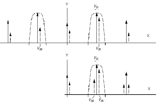
Intermodulation distortion is efficiently measured by applying one large tone (L1), performing a PSS analysis, and then applying the second small tone (S1) with a PAC analysis. In this case, the first tone drives the circuit hard enough to cause distortion and the second tone is used to measure only the intermodulation distortion. After V_L1, V_S1, and V_S3 are measured in dB at the output, the output third-order intercept point is computed using the following equation.

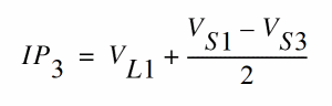
In the equation, V_L1, V_S1, and V_S3 must be given in some form of decibels. Currently, dBV is used in the Analog Circuit Design Environment. In this example, V_L1, V_S1, and VS3 are given in dBV. Consequently, the intercept point is also computed in dBV. If V_L1, V_S1, and V_S3 are given in dBm, the resulting intercept point is computed in dBm.

The intermodulation distortion of a mixer is measured in a similar manner, except that the PSS analysis must include both the LO and one large tone. For an example of measuring the intermodulation distortion of a mixer, see the Spectre Circuit Simulator and Accelerated Parallel Simulator RF Analysis in ADE Explorer User Guide.

If you must measure intermodulation distortion using two large tones to compare against bench measurements, you can run a PSS analysis with two large tones. However, a small commensurate frequency of the two tones can slow down simulation. At other times, use the quicker PSS/PAC approach.

For the PAC analysis the frequencies of the stimulus and response are usually different. This is an important difference between the PAC analysis and the AC analysis. The freqaxis parameter specifies whether the results should be output versus the input frequency, in, the output frequency, out, or the absolute value of the output frequency, absout.

You can make modulated small signal measurements using the Analog Circuit Design Environment (ADE). The modulated option for the PAC analysis and other modulated parameters are set in ADE. A PAC analyses with the modulated option produces results which might have limited use outside of ADE. The Direct Plot form is configured to analyze modulated small signal measurements and combine several waveforms to measure AM and PM response due to single sideband or modulated stimuli.

Frequency Sweep

You can specify sweep limits by providing either the end points or the center value and the span of the sweep.

Steps can be linear or logarithmic and you can specify either the number of steps or the size of each step. You can specify a step size parameter (step, lin, log, dec) to determine whether the sweep is linear or logarithmic. If you do not give a step size parameter, the sweep is linear when the ratio of stop to start values is less than 10:1, and logarithmic when this ratio is equal to or greater than 10:1.

Alternatively, you may specify particular values for the sweep parameter using the values parameter. If you give both a specific set of values and a set specified using a sweep range, the two sets are merged and collated before being used. All frequencies are in Hz.

Modulated Small-Signal Analyses

You can make modulated small signal measurements using the Analog Design Environment (ADE). The modulated option for PAC and other modulated parameters are set by ADE. PAC analyses with the modulated option produce results which might have limited use outside the ADE environment. The ADE Direct Plot form is configured to analyze these results and combine several wave forms to measure AM and PM response due to single sideband or modulated stimuli.

Sampled Small-Signal Analysis

Sampled small signal PXF and PAC analyses use the Analog Design Environment (ADE) environment. The sampled options are set by ADE. The Sampled option produces results which might have limited use outside ADE. Direct Plot is configured to analyze the results and make Sampled measurements due to single sideband or sampled stimuli. A sampled analysis is a small-signal analysis with a use model similar to the sampled (timedomain) PNoise analysis. Specifically, you first create a circuit (schematic or netlist description) and place port or source components to specify the key elements where the transfer function to the output is of interest.

The ability to sample the noise, signal slope and transfer function at a particular time point is a valuable investigative tool for design and verification. For example it will be used in a design of switched-capacitor filters, logic circuits and in the evaluation of the power supply rejection. A Sampled analysis computes the transfer function from different parts of the circuit to the output at a particular time point. The output signal is sampled at the clock rate (large signal period which is used in PSS).

A new choice in the Specialized Analysis cyclic menu, Sampled, opens the Sampled analysis fields in the Choosing Analyses form. Several fields are available to specify the sampling event. First, you select a control signal to observe in search for the triggering event(s). It could be a single or differential voltage signal or a probe, either voltage or current. The threshold value and the crossing direction are the parameters of a triggering timing event. In case of special need, you can specify a delayed measurement from the time of the crossing event.

You can also specify actual time points for sampling the output. The same form will be used and either one or the combination of both approaches is used to do the sampled small signal analysis.

Parameters for PAC Analysis

For information on PAC analysis parameters, refer to the Periodic AC Analysis (pac) section in the Spectre Circuit Simulator Reference manual

Periodic S-Parameter Analysis (PSP)

The Periodic S-Parameter (PSP) analysis is used to compute scattering and noise parameters for n-port circuits that exhibit frequency translation. Such circuits include mixers, switched-capacitor filters, samplers and other similar circuits.

PSP is a small-signal analysis similar to the conventional SP analysis, except, the circuit is first linearized about a periodically time-varying operating point as opposed to a simple DC operating point. Linearizing about a periodically time-varying operating point allows the computation of S-parameters between circuit ports that convert signals from one frequency band to another.

PSP analysis also calculates noise parameters in frequency-converting circuits. PSP computes noise figure (both single-sideband and double-sideband), input referred noise, equivalent noise parameters, and noise correlation matrices. The noise features of PSP analysis, as for Pnoise analysis but unlike SP analysis, include noise folding effects due to the periodically time-varying nature of the circuit.

Computing the n-port S-parameters and noise parameters of a periodically varying circuit is a two step process.

First, the small stimulus is ignored and the periodic steady-state response of the circuit to possibly large periodic stimulus is computed using PSS analysis.
As a normal part of the PSS analysis, the periodically time-varying representation of the circuit is computed and saved for later use.
Then, using the PSP analysis, small-signal excitations are applied to compute the n-port S-parameters and noise parameters.
A PSP analysis cannot be used alone, it must follow a PSS analysis. However, any number of periodic small-signal analyses such as PAC, PSP, PXF, and Pnoise, can follow a single PSS analysis.

Like other Spectre RF small-signal analyses, the PSP analysis can sweep only frequency.

PSP Synopsis

For a PSP analysis, you need to specify the port and port harmonic relations. Select the ports of interest by setting the port parameter. Set the periodic small-signal output frequencies of interest by setting the portharmsvec or the harmsvec parameters.

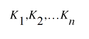
For a given set of n integer numbers representing the harmonics K₁, K₂, ... K_n, the scattering parameters at each port are computed at the frequencies

f(scattered)= f(rel) + K_i x fund(pss)

where f(rel) represents the relative frequency of a signal incident on a port, f(scattered) represents the frequency to which the relevant scattering parameter represents the conversion, and fund(pss) represents the fundamental frequency used in the corresponding PSS analysis.

Thus, when analyzing a down-converting mixer, with signal in the upper sideband, and sweeping the RF input frequency, the most relevant harmonic for RF input is Ki= 1 and for IF output Ki= 0. Hence we can associate K2=0 with the IF port and K1=1 with the RF port. S21 will represent the transmission of signal from the RF to IF, and S11 the reflection of signal back to the RF port. If the signal was in the lower sideband, then a choice of K1=-1 would be more appropriate.

You can use either the portharmsvec or the harmsvec parameters to specify the harmonics of interest. If you give portharmsvec, the harmonics must be in one-to-one correspondence with the ports, with each harmonic associated with a single port. If you specify harmonics with the optional harmsvec parameter, then all possible frequency-translating scattering parameters associated with the specified harmonics are computed.

For PSP analysis, the frequencies of the input and of the response are usually different (this is an important way in which PSP differs from SP). Because the PSP computation involves inputs and outputs at frequencies that are relative to multiple harmonics, the freqaxis and sweeptype parameters behave somewhat differently in PSP than they do in PAC and PXF.

The sweeptype parameter controls the way the frequencies are swept in PSP analysis. Specifying relative sweep, sweeps relative to the analysis harmonics (not the PSS fundamental). Specifying absolute sweep, sweeps the absolute input source frequency. For example, with a PSS fundamental of 100MHz, the portharmsvec set to [9 1] to examine a down-converting mixer, sweeptype=relative, and a sweep range of f(rel)=0->50MHz, then S21 would represent the strength of signal transmitted from the input port in the range 900-950MHz to the output port at frequencies 100->150MHz.

Using sweeptype=absolute and sweeping the frequency from 900->950MHz would calculate the same quantities, since f (abs)=900->950MHz, and f (rel) = f (abs) - K1 * fund(pss) = 0->50MHz, because K1=9 and fund(pss) = 100MHz.

The freqaxis parameter is used to specify whether the results should be output versus the scattered frequency at the input port(in), the scattered frequency at the output port(out) or the absolute value of the frequency swept at the input port(absin).

Unlike in PAC, PXF, and Pnoise analyses, increasing the number of requested ports and harmonics increases the simulation time substantially.

To ensure accurate results in PSP analysis, you should set the maxacfreq parameter for the corresponding PSS analysis to guarantee that |max{f(scattered)}| is less than the maxacfreq parameter value, otherwise the computed solution might be contaminated by aliasing effects.

PSP analysis also computes noise figures, equivalent noise sources, and noise parameters. The noise computation, which is skipped only when the donoise parameter is set to no, requires additional simulation time.

Noise Calculations Performed by PSP
Name	Description	Output Label
N_o	Total output noise at frequency f
Ns	Noise at the output due to the input probe (the source)
Nsi	Noise at the output due to the image harmonic at the source
Nso	Noise at the output due to harmonics other than input at the source
Nl	Noise at the output due to the output probe (the load)
IRN	Input referred noise	In
G	Gain of the circuit (See Note:)	Gain
F	Single sideband noise factor	F
NF	Single sideband noise figure	NF
Fdsb	Double sideband noise factor	F_dsb
NFdsb	Double sideband noise figure	NF_dsb
Fieee	IEEE single sideband noise factor	F_ieee
NFieee	IEEE single sideband noise figure	NF_ieee

The gain computed by PSP is the voltage gain from the actual circuit input to the circuit output, not the gain from the internal port voltage source to the output.

PSP analysis performs the following noise calculations.

Input referred noise

Single sideband noise factor

Single sideband noise figure

Double sideband noise factor

Double sideband noise figure

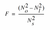
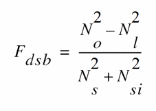
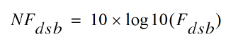
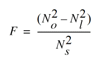
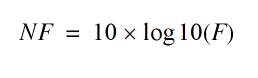
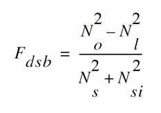
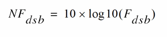
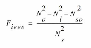
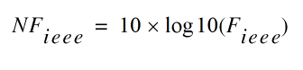
IEEE single sideband noise factor

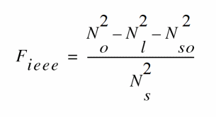
IEEE single sideband noise figure

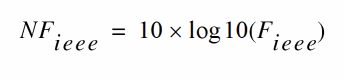
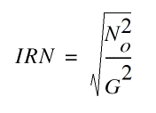
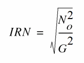
When the results are output, IRN is named in, G is named gain, F, NF, Fdsb, NFdsb, Fieee, and NFieee are named F, NF, Fdsb, NFdsb, Fieee, and NFieee, respectively.

To ensure accurate noise calculations, you need to set the maxsideband or sidebands parameters to include the relevant noise folding effects. The maxsideband parameter is only relevant to the noise computation features of PSP.

Parameters for PSP Analysis

For information on PSP analysis parameters, refer to the Periodic S-Parameter Analysis (psp) section in the Spectre Circuit Simulator Reference manual.

Periodic Transfer Function Analysis (PXF)

A conventional transfer function (XF) analysis computes the transfer function from every source in the circuit to a single output. An XF analysis differs from a conventional AC analysis in that the AC analysis computes the response from a single stimulus to every node in the circuit.

The difference between the PXF and PAC analyses is similar. The PXF analysis computes the transfer functions from any source at any frequency to a single output at a single frequency. Like PAC analysis, PXF analysis models frequency conversion effects. This is illustrated in Figure 2-4.

The PXF analysis directly computes such useful quantities as

Conversion efficiency (the transfer function from input to output at a desired frequency)
Image and sideband rejection (input to output at an undesired frequency)
LO feed-through and power supply rejection (undesired input to output at all frequencies)

PXF analysis measures conversion gains, especially those from the input source to the output. It also computes the conversion gain of the specified sideband as well as various unwanted images including the baseband feed through. PXF analysis also computes the coupling from other inputs such as the LO and the power supplies. These computations model frequency translation. PXF analysis determines the sensitivity of the output to either up-converted or down-converted noise from either the power supplies or the LO.

The output is sensitive to signals at many frequencies at the input of the mixer. The input signals are replicated and translated by each harmonic of the LO. The signals shown in Figure 2-4 are those that end up at the output frequency.

Computing transfer functions for a periodically varying circuit is a two step process.

First, the small stimulus is ignored and the periodic steady-state response of the circuit to possibly large periodic stimulus is computed using PSS analysis.
As a normal part of the PSS analysis, the periodically time-varying representation of the circuit is computed and saved for later use.
Second, using the PXF analysis, small-signal excitations are applied to compute the transfer functions.
Figure 2-4 Mixer Output Signals Shown by PXF Analysis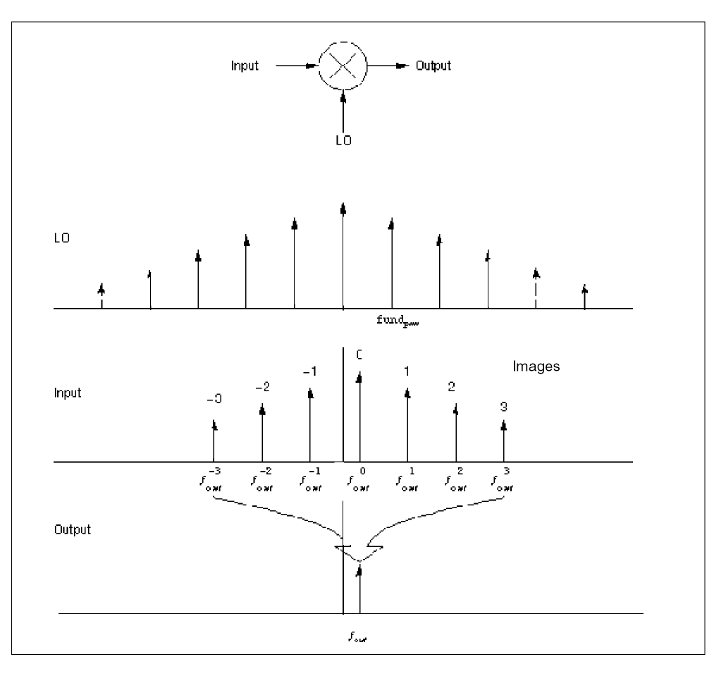

A PXF analysis cannot be used alone, it must follow a PSS analysis. However, any number of periodic small-signal analyses such as PAC, PSP, and Pnoise, can follow a single PSS analysis.

Unlike other Spectre RF small-signal analyses, the PXF analysis can sweep only frequency.

Parameters for PXF Analysis

For information on PXF analysis parameters, refer to the Periodic Transfer Function Analysis (pxf) section in the Spectre Circuit Simulator Reference manual.

Output Parameters

The output variable you measure can be voltage or current, and the variable frequency is not limited by the period of the large-periodic solution. When you sweep a selected output frequency, you can select the periodic small-signal input frequencies by specifying either one of the maxsideband or sideband parameters.

For a set of n integer numbers representing the sidebands

the input signal frequency at each sideband is computed as

where

f ( out ) represents the (possibly swept) output signal frequency
fund ( pss ) represents the fundamental frequency used in the corresponding PSS analysis

When you analyze a down-converting mixer and sweep the IF output frequency, k _i= +1 for the RF input represents the first upper sideband, and k _i= -1 for the RF input represents the first lower sideband. If you specify the maximum sideband value by setting the maxsideband value to k _max, you are selecting all 2 × k _max + 1 sidebands from - k _max to + k _max.

For PXF analysis, the number of sidebands you select with maxsideband does not substantially increase the simulation time. However, to ensure accurate PXF analysis results, set the maxacfreq parameter for the corresponding PSS analysis to guarantee that

otherwise the computed solution might be contaminated by aliasing effects. The PXF simulation does not run when

For these extreme cases, diagnostic messages indicate how you should change the maxacfreq parameter value in the PSS analysis. In a majority of simulations, however, this is not an issue because the maxacfreq value is never allowed to be smaller than 40 times the PSS fundamental.

With PXF analysis the frequency of the stimulus and response are usually different (this is an important way in which the PXF analysis differs from the XF analysis). Use the freqaxis parameter to specify whether the results should be output versus the input frequency, in, the output frequency, out, or the absolute value of the input frequency, absin.

Probe Parameters

You can specify the output with a pair of nodes or a probe component. Any component with two or more terminals can be a voltage probe. When there are more than two terminals, they are grouped in pairs. Use the portv parameter to select the appropriate pair of terminals. Alternatively, you can simply specify a voltage to be the output by giving a pair of nodes on the PXF analysis statement.

Any component that naturally computes current as an internal variable, such as a voltage source, can be a current probe. If the probe component computes more than one current, you use the porti parameter to select the appropriate current. Do not specify both the portv and porti parameters. If you do not specify either parameter, the probe component provides a reasonable default.

The Analog Circuit Design Environment (ADE) provides two ways to set probes on the Choosing Analyses form

When you specify input or output sources
When you specify positive or negative output nodes

Output Parameters

The stimuli parameter (on the PXF Options form) specifies the transfer function inputs. You select one of two choices:

Use stimuli = sources to use the sources present in the circuit. To compensate for gains or losses in the test fixture, use the xfmag source component parameter to adjust the computed gain to compensate for gains or losses in a test fixture. In hierarchical netlists, limit the number of sources using the save and nestlvl parameters.
Use stimuli = nodes_and_terminals to compute all possible transfer functions. Use this option when you cannot anticipate which transfer functions you might need to examine. This is useful when you do not know in advance which transfer functions are interesting.

Transfer functions for nodes are computed assuming that a unit magnitude flow (current) source is connected from the node to ground. Transfer functions for terminals are computed assuming that a unit magnitude value (voltage) source is connected in series with the terminal. By default, the PXF analysis computes the transfer functions from a small set of terminals.

For transfer functions from specific terminals, specify the terminals in the save statement. Use the :probe modifier (for example, Rout:1:probe) or specify useprobes=yes on the options statement. For transfer functions from all terminals, specify currents=all and useprobes=yes on the options statement.

Modulation Parameters

You can make modulated small-signal measurements from the Analog Circuit Design Environment (ADE). The modulated option for PXF analysis and other modulated parameters are set by ADE. The PXF analysis with the modulated option produces results which might have limited use outside the ADE environment. The Direct Plot form is configured to analyze modulated small-signal measurement results. Direct Plot can combine several wave forms to measure AM and PM transfer functions from single sideband or modulated stimuli to the specified output. For details, refer to the Spectre Circuit Simulator and Accelerated Parallel Simulator RF Analysis in ADE Explorer User Guide.

Sampled Small-Signal Analysis

You can also specify actual time points for sampling the output. The same form will be used and either one or the combination of both approaches is used to do the sampled small signal analysis.

Swept PXF Analysis

Specify sweep limits by providing either the end points (start and stop) or by providing the center value and the span (center and span) of the sweep.

Specify sweep steps as linear or logarithmic. Either specify the number of steps or the size of each step. You can give a step-size parameter (step, lin, log, dec) to determine whether the sweep is linear or logarithmic. If you do not give a step-size parameter, the sweep is linear when the ratio of stop to start values is less than 10, and logarithmic when this ratio is 10 or greater.

Alternatively, use the values parameter to specify the particular values that the sweep parameter should take. If you give both a specific set of values and a set of values specified using a sweep range, the two sets are merged and collated before being used. All frequencies are in Hertz.

Periodic Noise Analysis (Pnoise)

The Periodic Noise analysis (Pnoise) is similar to the conventional noise analysis except that it models frequency conversion effects. Hence Pnoise analysis is useful for predicting the noise behavior of mixers, switched-capacitor filters and other periodically driven circuits. The Pnoise analysis is particularly useful for predicting the phase noise of autonomous circuits, such as oscillators.

PNoise analysis linearizes the circuit about the periodic operating point computed in the prerequisite PSS analysis. It is the periodically time-varying nature of the linearized circuit that accounts for the frequency conversion. In addition, the affect of a periodically timevarying bias point on the noise generated by the various components in the circuit is also included.

Initially, PSS computes the response to a large periodic signal such as a clock or a LO. These results are labeled LO and shown in Figure 2-5. The subsequent Pnoise analysis computes the resulting noise performance.

In periodic systems, there are two effects that act to translate noise in frequency.

First, for noise sources that are bias dependent, such as shot noise sources, the time-varying operating point modulates the noise sources.
Second, the transfer function from the noise source to the output is also periodically time-varying and modulates the noise source contribution to the output.
Figure 2-5 How noise is moved around by a mixer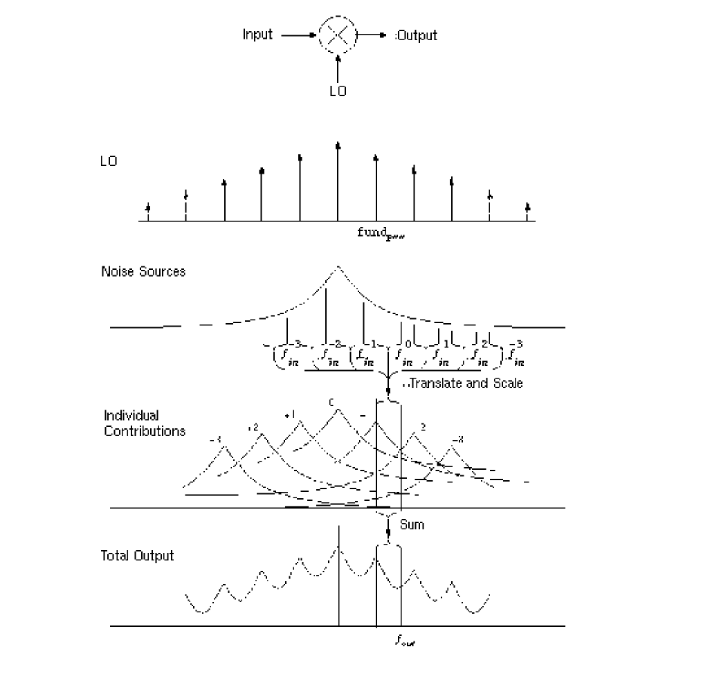

The time-average of the noise at the output is computed as a spectral density versus frequency. You identify the output by specifying a probe component or a pair of nodes. To specify the output with a probe, the preferred approach, use the oprobe parameter. If the output is voltage (or potential), choose a resistor or a port component for the output probe. If the output is current (or flow), choose a vsource or iprobe component for the output probe.

To compute the input-referred noise or the noise figure, specify the input source using the iprobe parameter. For input-referred noise, use either a vsource or isource as the input probe; for noise figure, use a port as the probe. Currently, only a vsource, an isource, or a port can be used as an input probe. If the input source is noisy, as is a port, the noise analysis will compute the noise factor (F) and noise figure (NF). To match the IEEE definition of noise figure, the input probe must be a port with no excess noise and its noisetemp must be set to 16.85C (290K). In addition, the output load must be a resistor or port and must be identified as the oprobe.

If port is specified as the input probe, then both input-referred noise and gain are referred back to the equivalent voltage source inside the port. S-parameter analysis calculates those values in the traditional sense.

The reference sideband (refsideband) specifies which conversion gain is used to compute the input-referred noise, the noise factor, and the noise figure. The reference sideband specifies the input frequency relative to the output frequency with

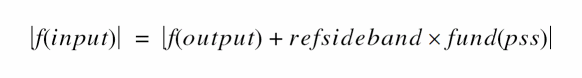
Use refsideband=0 when the input and output of the circuit are at the same frequency, such as with amplifiers and filters. When refsideband does not equal 0, the single sideband noise figure is computed.

The Pnoise analysis computes the total noise at the output, which includes contributions from the input source, the circuit itself and the output load. The amount of the output noise that is attributable to each noise source in the circuit is also computed and output individually. If the input source is identified (using iprobe) and is a vsource or isource, the input-referred noise is computed, which includes the noise from the input source itself. Finally, if the input source is identified (using iprobe) and is also noisy, as is the case with ports, the noise factor and noise figure are computed.

Noise Calculations Performed by Pnoise
Name	Description	Output Label
N_o	Total output noise	Out
Ns	Noise at the output due to the input probe (the source)
Nsi	Noise at the output due to the image harmonic at the source
Nso	Noise at the output due to harmonics other than input at the source
Nl	Noise at the output due to the output probe (the load)
IRN	Input referred noise	In
G	Gain of the circuit	Gain
F	Single sideband noise factor	F
NF	Single sideband noise figure	NF
Fdsb	Double sideband noise factor	F_dsb
NFdsb	Double sideband noise figure	NF_dsb
Fieee	IEEE single sideband noise factor	F_ieee
NFieee	IEEE single sideband noise figure	NF_ieee

Spectre RF performs the following noise calculations.

Input referred noise

Single sideband noise factor

Single sideband noise figure

Double sideband noise factor

Double sideband noise figure

IEEE single sideband noise factor

IEEE single sideband noise figure

Pnoise Synopsis

Noise can mix with each harmonic of the periodic drive signal from the PSS analysis and appear at the output frequency. However, Pnoise analysis models only noise that mixes with a set of harmonics that you normally specify with the maxsideband parameter, but which you might specify with the sidebands parameter in special circumstances. If Ki represents sideband i, then

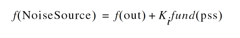
The maxsideband parameter specifies the maximum |Ki| included in the Pnoise calculation. Therefore, Pnoise ignores noise at frequencies less than f(out) – maxsideband fund (pss) and greater than f(out) + maxsideband fund (pss). If you specify sidebands with the sidebands parameter, then Pnoise includes only the specified sidebands in the calculation. When you specify sidebands parameter values, be careful not to omit any sidebands that might contribute significant output noise.

In practice, noise can mix with each of the harmonics of the periodic drive signal applied in the PSS analysis and end up at the output frequency. However, the PNoise analysis only includes the noise that mixes with a finite set of harmonics that are typically specified using the maxsideband parameter, but in special circumstances may be specified with the sidebands parameter. If Ki represents sideband i, then

f (noise_source) = f (out) + Ki * fund(pss)

The maxsideband parameter specifies the maximum |Ki| included in the PNoise calculation. Thus, noise at frequencies less than f(out)-maxsideband*fund(pss) and greater than f(out)+maxsideband*fund(pss) are ignored. If selected sidebands are specified using the sidebands parameter, then only those are included in the calculation. You should take care when specifying the sidebands because the results will be in error if you do not include a sideband that contributes significant noise to the output.

The number of requested sidebands does not change substantially the simulation time. However, the maxacfreq of the corresponding PSS analysis should be set to guarantee that |max{f(noise_source)}| is less than maxacfreq, otherwise the computed solution might be contaminated by aliasing effects. The PNoise simulation is not executed for |f(out)| greater than maxacfreq. Diagnostic messages are printed for those extreme cases, indicating which maxacfreq should be set in the PSS analysis. In the majority of the simulations, however, this is not an issue, because maxacfreq is never allowed to be smaller than 40 times the PSS fundamental.

Phase Noise measurements are possible using the Analog Design Environment (ADE). Two Pnoise analyses are preconfigured for this simulation and most of the parameters are set by ADE.

The mod1 Pnoise analysis is a regular noise analysis and can be used independently.
The mod2 Pnoise analysis is a correlation analysis and has limited use outside of the ADE environment.

The Direct Plot form in ADE is configured to analyze these results and combine several waveforms to measure AM and PM components of output noise.

You can specify sweep limits by giving the end points or by providing the center value and the span of the sweep. Steps can be linear or logarithmic, and you can specify the number of steps or the size of each step. You can give a step size parameter (step, lin, log, dec) to determine whether the sweep is linear or logarithmic. If you do not give a step size parameter, the sweep is linear when the ratio of stop to start values is less than 10, and logarithmic when this ratio is 10 or greater. Alternatively, you may specify the particular values that the sweep parameter should take using the values parameter. If you give both a specific set of values and a set specified using a sweep range, the two sets are merged and collated before being used. All frequencies are in Hz.

Parameters for Pnoise Analysis

For information on pnoise analysis parameters, refer to the Periodic Noise Analysis (pnoise) section in the Spectre Circuit Simulator Reference manual.

Noise Figure

When you use Pnoise analysis to compute the noise factor or noise figure of a circuit, and the load generates noise, specify the output with the oprobe parameter rather than using a pair of nodes. Using the oprobe parameter explicitly specifies the load as the output probe. This is preferable because it excludes the noise of the load from the calculation of the noise figure.

As an alternative, you can specify the output with a pair of nodes and make the load component a noiseless resistor. Results with this approach are similar to those computed if you specify a resistor or a port as the output probe (load). The only difference is that the noiseless resistor is considered noiseless for other noise calculations, such as total output noise and input-referred noise, and the resistor is noiseless at all frequencies. When you specify a conventional resistor or port for the load, its noise is subtracted from only the noise factor and noise figure calculations, and only at the output frequency. Consequently, noise from load frequencies other than the output frequency can appear at the output frequency if the circuit has a nonlinear output impedance.

Pnoise computes the single-sideband noise figure. To match the IEEE definition of noise figure, you must use a port as the input probe and a resistor or a port as the output probe. In addition, the input port noise temperature must be 290 K (noisetemp = 16.85) and have no excess noise. (You must not specify noisevec and noisefile on the input port.) The 290K temperature is the average noise temperature of an antenna used for terrestrial communication. However for your application, you can specify the input port noise temperature to be any appropriate value. For example, the noise temperature for antennas pointed at satellites is usually much lower.

Frequency-Aware PPV Analysis for Oscillators with Large Time Constants

Phase noise, because it has an impact on overall system performance, is a major concern in oscillator circuit design. The perturbation projection vector (PPV) models often used to analyze oscillators overestimate the phase noise in oscillators with large time constants, such as oscillators that include switch capacitors, DC bias, or digital dividers. The overestimation error happens because the slow nodes in oscillators filter out the noise from nearby devices and the PPV does not consider these filtering effects.

Setting the augmented parameter to yes turns on an analysis that considers the PPV as a frequency dependent quantity. This frequency-aware analysis takes into account the fact that different perturbation frequencies have different PPV waveforms. The analysis provides the same answers as ordinary PPV analysis for small, fast oscillators but provides a more accurate result for oscillators with large time constants.

Flicker Noise

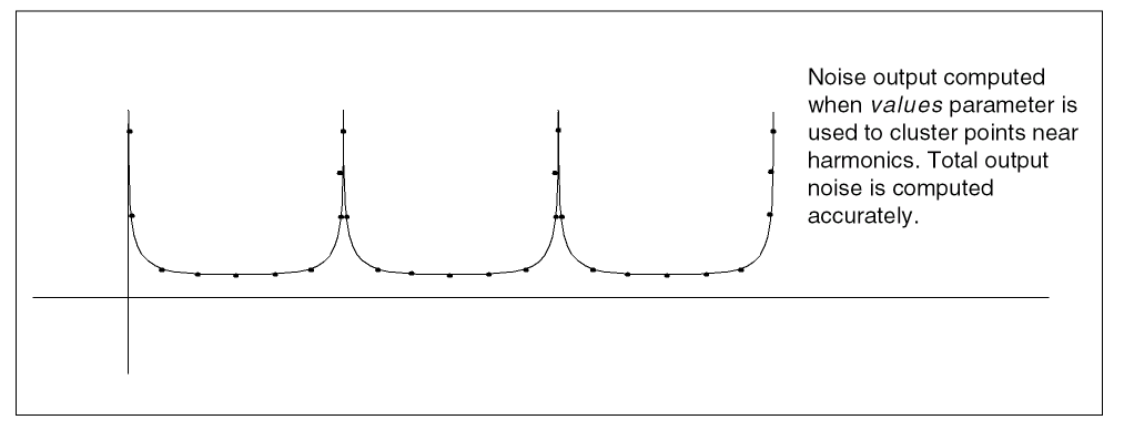
To avoid inaccurate results with Pnoise analysis on a circuit that mixes flicker noise or 1/f noise up to the carrier or its harmonics, place a cluster of frequencies near each harmonic to resolve the noise peaks accurately, but do not put frequency points precisely on the harmonics. In addition, choose Pnoise start and stop frequencies to avoid placing points precisely on the harmonics of the periodic drive signal. Then use the values parameter to specify a vector of additional frequency points near the harmonics. In the Analog Circuit Design Environment, the values parameter is set in the Add Specific Points field in the Choosing Analyses form.

The effect of specifying appropriate additional frequency points is shown in the following three diagrams. Figure 2-6 shows the true output noise of a mixer with flicker noise.

Figure 2-6 Actual Mixer Noise Output Including Flicker Noise

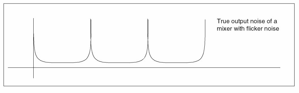
Figure 2-7 shows the output noise computed with a typical choice of points. In this case, total output noise is typically exaggerated by many orders of magnitude.

Figure 2-7 Noise Output Computed With Typical Points

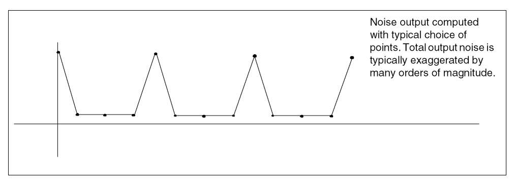
Figure 2-8 shows noise output computed when the values parameter is used to cluster points near harmonics. By comparing Figures 2-7 and 2-8, you can see that total output noise is computed accurately when points are carefully chosen.

Figure 2-8 Noise Output Computed With Clustered Points

Flicker Noise Spectrum

Flicker noise depends on the current, I, of the channel. For all devices, flicker, or 1/f, noise depends on the following equation

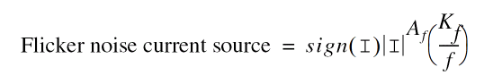
This means that you see only odd harmonics. The power looks like a rectified sine wave because

Periodic Stability Analysis (PSTB)

The periodic stability (PSTB) analysis evaluates the local stability of a periodically time-varying feedback circuit. It is a small-signal analysis, like STB analysis, except that the circuit is first linearized about a periodically varying operating point as opposed to a simple DC operating point. Linearizing about a periodically time-varying operating point allows the stability evaluation to include the effect of the time-varying operating point.

The stability evaluation of a periodically varying circuit is a two step process.

First, the small stimulus is ignored and the periodic steady-state response of the circuit to a possibly large periodic stimulus is computed using PSS analysis. As a normal part of the PSS analysis, the periodically time-varying representation of the circuit is computed and saved for later use.
Then, the small stimulus is applied to compute the loop gain of the zero sideband with a probe component. The local stability can be evaluated using gain margin, phase margin, or a Nyquist plot of the loop gain. To perform PSTB analysis, you must use a probe instance and specify it with the probe parameter.

The loop-based algorithm requires that you place the probe on the feedback loop to identify and characterize the particular loop of interest. The introduction of the probe component should not change any of the circuit characteristics. Because of the time-varying properties of the circuit, the loop gain at different places might be different but you can use the loop gain at any point to evaluate stability.

The loop-based algorithm provides stability information for both single loop circuits and for multi-loop circuits in which you can place a probe component on a critical wire to break all loops. For a general multi-loop circuit, such a critical wire might not be available. The loop-based algorithm can only be performed on individual feedback loops to ensure they are stable.

The device based algorithm requires the probe be a gain instant, such as a bjt transistor or a mos transistor. The device-based algorithm evaluates the loop gain around the probe, which can be involved in multi-loops.

Unlike other analyses in Spectre RF, this analysis can only sweep frequency.

Parameters for PSTB Analysis

For information on PSTB analysis parameters, refer to the Periodic STB Analysis (pstb) section in the Spectre Circuit Simulator Reference manual.

Sweep

You can specify sweep limits by providing

The end points of the sweep
The center value and the span of the sweep
An array of specific values to sweep

Steps can be linear or logarithmic and you can specify either the number of steps or the size of each step. You can specify a step size parameter (step, lin, log, dec) to determine whether the sweep is linear or logarithmic. If you do not provide a step size parameter, the sweep is linear when the ratio of stop to start values is less than 10:1 and logarithmic when this ratio is equal to or greater than 10:1.

Alternatively, you may specify particular values for the sweep parameter using the values parameter. If you give both a specific set of values and a set specified using a sweep range, the two sets are merged and collated before being used. All frequencies are in Hertz.

Understanding Loop-Based and Device-Based Algorithms

Both loop-based and device-based algorithms are available for periodic small-signal stability analysis. When the probe parameter points to a current probe or voltage source instance, the loop-based algorithm is used; when it points to a supported active device instance, the device-based algorithm is used.

About the PSTB Loop-Based Algorithm

The PSTB loop-based algorithm is based on a subset of Nyquist criteria. The analysis outputs the loop gain waveform.

The PSTB loop-based algorithm calculates the true loop gain, which consists of both normal loop gain and reverse loop gain. The loop-based algorithm requires that you place a probe component in the feedback loop to identify and characterize the particular loop of interest. Introducing the probe component should not change circuit characteristics.

The loop-based algorithm provides accurate stability information for single loop circuits. It also provides accurate stability information for multi-loop circuits in which you can place a probe component on a critical wire to break all loops. For general multi-loop circuits, such a critical wire may not be available. The loop-based algorithm can only be performed on individual feedback loops to ensure they are stable. Although the stability of all feedback loops is a necessary condition for the whole circuit to be stable, the multi-loop circuit tends to be stable if all individual loops are associated with reasonable stability margins.

Device-Based Algorithm

The device-based algorithm calculates the loop gain around a particular active device, which must be a gain instance such as a bjt or mos transistor. This algorithm is often applied to assess the stability of circuit designs in which local feedback loops cannot be neglected. The loop-based algorithm cannot be used for such designs because the local feedback loops are inside the devices where a probe component cannot be inserted.

When the probe parameter points to a particular active device, the dominant controlled source in the device is nulled during the analysis. The device-based algorithm produces accurate stability information for a circuit in which a critical active device can be identified such that nulling the dominant gain source of this device renders the whole network to be passive.

Quasi-Periodic Steady-State Analysis (QPSS)

The quasi-periodic steady-state (QPSS) analysis computes the quasi-periodic steady-state response of a circuit that operates on multiple time scales. A quasi-periodic signal has dynamics in multiple fundamental frequencies. Closely spaced or incommensurate fundamentals cannot be efficiently resolved by PSS analysis. (Incommensurate frequencies are those for which there is no period that is an integer multiple of the period of each frequency.) QPSS analysis allows you to compute circuit responses to several moderately large input signals in addition to a strongly nonlinear tone which represents the LO or clock signal. A typical example is the intermodulation distortion measurements of a mixer with two closely spaced moderate input signals. QPSS treats one particular input signal (usually the one that causes the most nonlinearity or the largest response) as the large signal, and the others as moderate signals.

When you perform a QPSS analysis

An initial transient analysis runs with all moderate input signals suppressed.
A number of stabilizing iterations run (always at least 2) with all signals activated.
The shooting Newton method runs.

The QPSS analysis using the shooting engine employs the Mixed Frequency Time (MFT) algorithm extended to multiple fundamental frequencies. For details about the MFT algorithm, see Steady-State Methods for Simulating Analog and Microwave Circuits, by K. S. Kundert, J. K. White, and A. Sangiovanni-Vincentelli, Kluwer, Boston, 1990.

Like PSS analysis, QPSS analysis uses the shooting Newton method as its backbone. However, unlike PSS analysis (where each Newton iteration performs a single transient integration), for each Newton iteration the QPSS analysis performs a number of transient integrations of one large signal period. Each integration differs by a phase-shift in each moderate input signal. When you set up a QPSS analysis, you determine the number of integrations performed by the number of harmonics of moderate fundamentals you select.

You select the moderate signals to model with the maxharms parameter as follows

QPSS always treats k1 as the maximum harmonic of the large signal and the total number of integrations for the simulation is calculated as

One consequence is that the efficiency of the algorithm depends significantly on the number of harmonics required to model the responses of moderate fundamentals. Another consequence is that the number of harmonics of the large fundamental does not significantly affect the efficiency of the shooting algorithm. The boundary conditions of a shooting interval are such that the time domain integrations are consistent with a frequency domain transformation with a shift of one large signal period.

Comparing QPSS Analysis with PSS and PAC Analyses

A QPSS analysis is similar to a PSS analysis followed by a PAC analysis in that if you treat one of the input signals as a small signal, a signal whose harmonics do not contribute significantly to the output, you can use the PSS/PAC analyses to model intermodulation distortion effectively.

The QPSS analysis has the following advantages that make it the analysis of choice in many situations. For example, with a QPSS analysis you can measure

Harmonic distortion and frequency translation effects created by multiple moderate-signal inputs, including all third order products. These measurements are impossible to obtain using PSS/PAC analysis because they do not model the effects of small-signal harmonics.
The effects of multiple moderate signals. With PSS/PAC analysis, you are restricted to modeling the effects of a single small signal on the fundamental you compute with the PSS analysis. A QPSS analysis lets you model all moderate-signal inputs, including the sums of sinusoids that are not periodic.

To see the difference between the information available with QPSS and PSS/PAC analyses, compare how the two approaches determine the output signals produced by input signals at 900 MHz and 905 MHz. The discussion below assumes you are interested in data only for fundamentals and their first harmonics.

If you perform a PSS analysis for the 900 MHz signal followed by a PAC analysis that applies 905 MHz as a small-signal with maxsideband = k1, you get

Where

If you perform a QPSS analysis with input signals at 900 MHz (for the large tone) and 905 MHz (for the moderate tone), you get information about the following additional frequency translation signals created by moderate tones.

The output signals are centered at the following frequencies:

where

and

Again, the number of harmonics of the moderate tone ( k ₂) effects the simulation time.

Figure 2-9 shows that more information is available from a QPSS analysis than from a PSS analysis followed by a PAC analysis.

Figure 2-9 Comparison of Information From QPSS and PSS/PAC Analyses

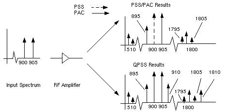
QPSS Parameters

For information on QPSS analysis parameters, refer to the Quasi-Periodic Steady State Analysis (qpss) section in the Spectre Circuit Simulator Reference manual.

The QPSS analysis uses the same parameters as the PSS analysis with a couple of parameters added and a few parameters extended. The most important parameters for QPSS analysis are the funds and maxharms parameters, which replace and extend the fund (or period) and harms parameters that are used in PSS analysis.

The funds parameter accepts a list of names of fundamentals that are present in the sources. (These fundamental names are specified by the source parameter fundname.) The simulator automatically figures out the frequencies associated with the fundamental names. An important feature of the funds parameter is that each input signal can be composed of more than one source, provided that all the sources have the same fundamental name. The fundamental frequency for each fundamental name is the greatest common factor of all the frequencies associated with the name. Simulation terminates if you do not list all the fundamental names on the funds parameter.

If you do not specify maxharms, a warning message displays, and the number of harmonics defaults to 1 for each fundamental.

The first fundamental is considered the large signal. You can use a few heuristics to pick the large fundamental.

Pick the fundamental that is not sinusoidal.
Pick the fundamental that causes the most nonlinearity.
Pick the fundamental that causes the largest response.

The maxharms parameter accepts a list of numbers of harmonics that are required to sufficiently model responses due to different fundamentals.

The role of some PSS parameters is extended for QPSS analysis.

The maxperiods parameter that controls the maximum number of shooting iterations for PSS analysis also controls the maximum number of shooting iterations for QPSS analysis. Its default value is 50. The tstab parameter controls both the length of the initial transient integration, with only the clock tone activated, and the number of stabilizing iterations, with the moderate tones activated. The stable iterations are run before Newton iterations begin.

The errpreset Parameter in QPSS Analysis

The errpreset parameter quickly adjusts several simulator accuracy parameters to fit your needs.

In most cases, errpreset should be the only accuracy parameter you need to adjust.

For a fast simulation with reasonable accuracy, set errpreset to liberal.
For greater accuracy, set errpreset to moderate.
If accuracy is your primary concern, set errpreset to conservative.

If you do not specify a value for steadyratio, it is always 1.0, and it is not affected by errpreset.

Table 2-5 shows the effect of errpreset settings (liberal, moderate, and conservative) on the default values of a set of accuracy parameters.

Table 2-5 Parameter Default Values for `errpreset` Settings

errpreset	reltol	relref	method	Iteratio	maxstep
`liberal`	1e^-3	sigglobal	gear2only	3.5	clock period/80
`moderate`	1e^-4	sigglobal	gear2only	3.5	clock period/100
`conservative`3	1e^-5	sigglobal	gear2only	*	clock period/200

These errpreset settings include a default reltol value which is an enforced upper limit for reltol. An increase of reltol above the default is ignored by the simulator. The only way to decrease the reltol value is in the options statement. The only way to increase the reltol value is to relax the errpreset setting. Spectre RF sets the maxstep parameter value so that it is no larger than the value given in Table 2-5.

With the exception of the reltol and maxstep values, the errpreset setting does not change any parameter values you have explicitly set. The actual values used for the QPSS analysis are given in the log file. If errpreset is not specified in the netlist, liberal settings are used.

For HB, only reltol is affected by errpreset, and the effect is the same as that in shooting. However, lteratio remains 3.5 and steadyratio remains 1 with all values of errpreset.

With parameter hbhomotopy, you can specify harmonic balance homotopy selection methods. The possible values of parameter hbhomotopy and their meanings are as follows:

hbhomotopy=tstab: Simulator runs a transient analysis and generates an initial guess for harmonic balance analysis; it is recommended for nonlinear circuits or circuits with frequency dividers.

hbhomotopy=source: For driven circuit, simulator ignores tstab and accordingly increases the source power level; for oscillators, the simulator accordingly adjusts the probe magnitude until the probe has no effect on the oscillators. It is recommended for strongly nonlinear or high Q circuits.

hbhomotopy=tone: This method is valid only for multi-tone circuit. The simulator first solves a single-tone circuit by turning off all the tones except the first one, and then solves the multitone circuit by restoring all the tones and using the single-tone solution as its initial guess; it is recommended for multi-tone simulation with a strong first tone.

hbhomotopy=inctone: Simulator first solves a single tone, then turns on moderate tones incrementally till all tones are enabled. It is recommended for circuits with one strong large tone.

hbhomotopy=gsweep: A resistor, whose conductance is g, is connected with each node, and the sweep of g is controlled by gstart, gstop, and glog. It is recommended for circuits containing high-impedance or quasi-floating nodes.

Quasi-Periodic Noise Analysis (QPnoise)

The Quasi-Periodic Noise (QPnoise) analysis is a quasi-periodic small-signal analysis similar to the conventional noise analysis, except that with QPnoise the circuit is first linearized about a quasi-periodically time-varying operating point as opposed to a simple DC operating point. Linearizing about a quasi-periodically time-varying operating point includes frequency conversion and intermodulation effects. Simply linearizing about a DC operating point cannot include frequency translation because linear time-invariant circuits do not exhibit frequency translation. QPnoise also includes the effect of a quasi-periodically time-varying bias point on the noise generated by the various components in the circuit. Hence QPnoise is useful for predicting the noise behavior of mixers, switched-capacitor filters, and other periodically or quasi-periodically driven circuits. You cannot use a QPnoise analysis alone. It must follow a QPSS analysis. However, any number of quasi-periodic small signal analyses (QPAC, QPSP, QPXF, and QPnoise) can follow a single QPSS analysis.

Computing the small-signal response of a quasi-periodically varying circuit is a two step process.

First, the small stimulus is ignored and the quasi-periodic steady-state response of the circuit to possibly large periodic stimuli is computed with a QPSS analysis. As a normal part of the QPSS analysis, the quasi-periodically time-varying representation of the circuit is computed and saved for later use.
Then, the small stimuli representing both individual noise sources in the circuit as well as the input noise are applied to the periodically-varying linear representation to compute the small signal response. This is done using the QPnoise analysis.

QPnoise Output

The time-average of the noise at the output of the circuit is computed in the form of a spectral density versus frequency. The output of the circuit is specified with either a pair of nodes or a probe component. To specify the output of a circuit with a probe, specify it using the oprobe parameter. If the output is voltage (or potential), choose a resistor or a port as the output probe. If the output is current (or flow), choose a vsource or iprobe as the output probe.

If you want the input-referred noise, specify the input source using the iprobe parameter. Currently, only a vsource, an isource, or a port can be used as an input probe. If the input source is noisy, as is a port, the noise analysis will compute the noise factor (F) and noise figure (NF). To match the IEEE definition of noise figure, the input probe must be a port with no excess noise and you must set its noisetemp parameter to 16.85 C (290 K). In addition, the output load must be a resistor or port and must be identified as the oprobe.

If port is specified as the input probe, then both input-referred noise and gain are referred back to the equivalent voltage source inside the port. S-parameter analysis calculates those values in traditional sense.

Use the refsideband parameter to specify which conversion gain to use when computing input-referred noise, noise factor, and noise figure. The reference sideband satisfies:

The reference sideband option (refsidebandoption) specifies whether to consider the input at the frequency or the input at the individual quasi-periodic sideband specified. Note that different sidebands can lead to the same frequency.

Sidebands are vectors in QPnoise analysis. Assume you have one large tone and one moderate tone in a QPSS analysis. A sideband Ki will be a vector [Ki_1 Ki_2]. It gives the frequency at

Ki_1 * fund(large tone of QPSS) + Ki_2 * fund(moderate tone of QPSS)

Use refsideband=[0 0...] when the input and output of the circuit are at the same frequency (such as with amplifiers and filters). When the refsideband parameter value differs from the 0 vector, QPnoise computes the single side-band noise figure.

The noise analysis always computes

Total noise at the output. This includes contributions from the input source and the output load.
The amount of output noise that is attributable to each noise source in the circuit. These are computed and output individually.

If you identify the input source with iprobe and it is a vsource or an isource, the input-referred noise is computed. This includes the noise from the input source itself.

If you identify the input source with iprobe and it is noisy, as is the case with ports, the noise factor and noise figure are computed.

Noise Calculations Performed by QPnoise
Name	Description	Output Label
N_o	Total output noise	Out
Ns	Noise at the output due to the input probe (the source)
Nsi	Noise at the output due to the image harmonic at the source
Nso	Noise at the output due to harmonics other than input at the source
Nl	Noise at the output due to the output probe (the load)
IRN	Input referred noise (See Note:)	In
G	Gain of the circuit (See Note:)	Gain
F	Single sideband noise factor	F
NF	Single sideband noise figure	NF
Fdsb	Double sideband noise factor	F_dsb
NFdsb	Double sideband noise figure	NF_dsb
Fieee	IEEE single sideband noise factor	F_ieee
NFieee	IEEE single sideband noise figure	NF_ieee

For the QPnoise analysis, the computation of gain and IRN assumes that the circuit under test is impedance-matched to the input source. This can introduce inaccuracy into the gain and IRN computation.

Spectre RF performs the following noise calculations.

Input referred noise

Single sideband noise factor

Single sideband noise figure

Double sideband noise factor

Double sideband noise figure

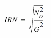
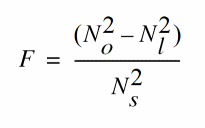
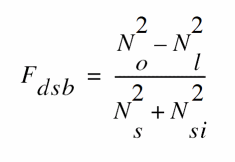
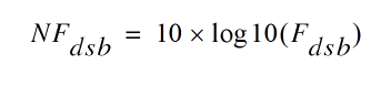
IEEE single sideband noise factor

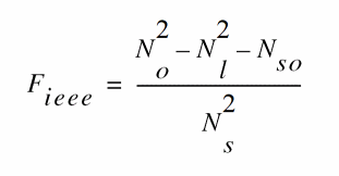
IEEE single sideband noise figure

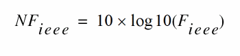
QPnoise Synopsis

At the UNIX command line use the optional terminals (p and n) to specify the output of the circuit. If you do not give the terminals, then you must specify the output with a probe component.

In practice, noise can mix with each of the harmonics of the quasi-periodic drive signals applied in the QPSS analysis and end up at the output frequency. However, the QPnoise analysis includes only the noise that mixes with a finite set of harmonics that are specified using the clockmaxharm and sidevec parameters.

The clockmaxharm parameter affects only clock frequency. It can be less or more than maxharms[1] in QPSS. Moderate tones are limited by maxharms specified in QPSS. Only the selected sidebands specified using the sidevec parameter are included in the calculation. Care should be taken when specifying sidevec or clockmaxharm in QPNOISE and maxharms in QPSS. Noise results are erroneous if you do not include the sidebands that contribute significant noise to the output.

The number of requested sidebands will substantially change the simulation time.

In quasi-periodic analyses sidebands are vectors, or, in other words, harmonic combinations. One way to specify them is using the sidevec parameter. When a QPSS analysis has one large tone and one moderate tone, the sideband is represented by a vector K¹ as [K¹₁ K¹₂]. The corresponding frequency translation is

When there are L tones total in the QPSS analysis (1 large tone and L-1 moderate tones), there is also a given set of n integer vectors representing the sidebands

K¹ = { K¹₁, ..., K¹_j,..., K¹_L} K² = { K²₁, ..., K²_j,..., K²_L} … Kⁿ = { Kⁿ₁, ..., Kⁿ_j,..., Kⁿ_L}

The QPnoise analysis computes the output frequency corresponding to each sideband as follows.

where

f(in) represents the (possibly swept) input frequency
f _j represents the fundamental frequency used in the corresponding QPSS analysis.

Enter the sidevec parameter as a sequence of integer numbers separated by spaces. For example, you would enter the set of vectors {1 1 0} {1 -1 0} {1 1 1} as follows

sidevec=[ 1 1 0 1 -1 0 1 1 1]

The other way to specify the sidebands is the clockmaxharm parameter and the maxharms parameter in the preceding QPSS analysis. Only the large tone, the first fundamental in QPSS, is affected by the QPnoise clockmaxharm parameter value. It limits the maximum harmonic order of the large tone that will be considered. All the remaining tones, the moderate tones, are limited by the QPSS maxharms parameter value.

Given the following parameters

In the QPSS analysis input, maxharms=[k⁰_max k²_max... kⁿ_max]
In the QPnoise analysis input, clockmaxharm=K_max

The QPnoise analysis output generates the following number of sidebands

(2*Kmax + 1)*(2*k²max+1)*(2*k³max+1)*...*(2*kⁿmax+1)

Swept QPnoise Analysis

Specify sweep limits by providing either the end points (start and stop) or by providing the center value and the span of the sweep (center and span).

Specify sweep steps as linear or logarithmic as well as the number of steps or the size of each step. You can give a step-size parameter (step, lin, log, dec) to determine whether the sweep is linear or logarithmic. If you do not give a step-size parameter, the sweep is linear when the ratio of stop to start values is less than 10:1, and logarithmic when this ratio is equal to or greater than 10:1.

Alternatively, you can specify the particular values for the sweep parameter using the values parameter. If you give both a specific set of values and a set specified using a sweep range, the two sets are merged and collated before simulation. All frequencies are in Hertz.

QPnoise Parameters

For information on QPnoise analysis parameters, refer to the Quasi-Periodic Noise Analysis (qpnoise) section in the Spectre Circuit Simulator Reference manual.

Quasi-Periodic AC Analysis (QPAC)

The quasi-periodic AC (QPAC) analysis computes transfer functions for circuits that exhibit multitone frequency translation. Such circuits include mixers, switched-capacitor filters, samplers, phase-locked loops, and similar circuits.

QPAC is a quasi-periodic small-signal analysis like the conventional AC analysis, except that with QPAC the circuit is first linearized about a quasi-periodically time-varying operating point as opposed to a simple DC operating point. Linearizing about a quasi-periodically time-varying operating point produces transfer-functions that include frequency translation. Simply linearizing about a DC operating point cannot include frequency translation because linear time-invariant circuits do not exhibit frequency translation.

Computing the small-signal response of a quasi-periodically varying circuit is a two step process.

First, the small stimulus is ignored and the quasi-periodic steady-state response of the circuit to possibly large periodic stimuli is computed with a QPSS analysis. As a normal part of the QPSS analysis, the quasi-periodically time-varying representation of the circuit is computed and saved for later use.
Second, the small stimuli are applied to the periodically-varying linear representation to compute the small signal response. This is done using the QPAC analysis.

QPAC Output Frequency and Sideband Vectors

You select the set of quasi-periodic small-signal output frequencies you are interested in by setting either the clockmaxharm or the sidevec output parameters.

In quasi-periodic analyses sidebands are vectors, or, in other words, harmonic combinations. One way to specify them is using the sidevec parameter. When a QPSS analysis has one large tone and one moderate tone, the sideband is represented by the vector K¹ as [K¹₁ K¹₂]. The corresponding frequency translation is

When there are L tones total in the QPSS analysis (1 large tone and L-1 moderate tones), there is also a given set of n integer vectors representing the sidebands

K¹ = { K¹₁, ..., K¹_j,..., K¹_L} K² = { K²₁, ..., K²_j,..., K²_L} … Kⁿ = { Kⁿ₁, ..., Kⁿ_j,..., Kⁿ_L}

The QPAC analysis computes the output frequency corresponding to each sideband as follows.

Where

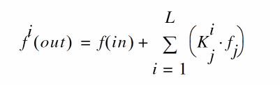
f(in) represents the (possibly swept) input frequency
f _j represents the fundamental frequency used in the corresponding QPSS analysis.

In modeling a down-converting mixer with low-side LO and with swept RF input frequency, the most relevant sideband for the IF output is {-1,0}. For an up-converting mixer with swept IF input frequency, the most relevant sideband for the RF output is {1,0}. In a typical IP3 measurement, IM1 will correspond to the {-1, 0} sideband and IM3 to the {-1, 2} sideband.

Enter the sidevec parameter as a sequence of integer numbers separated by spaces. For example, you would enter the set of vectors {1 1 0} {1 -1 0} {1 1 1} as follows

sidevec=[ 1 1 0 1 -1 0 1 1 1]

The other way to specify the sidebands is the clockmaxharm parameter and the maxharms parameter in the preceding QPSS analysis. Only the large tone, the first fundamental in QPSS, is affected by the clockmaxharm parameter value. It limits the maximum harmonic order of the large tone that will be considered. All the remaining tones, the moderate tones, are limited by the QPSS maxharms parameter value.

Given the following parameters

maxharms=[k¹_max k²_max... kⁿ_max]
clockmaxharm=K_max

The following sidebands are generated:

(2*Kmax + 1)*(2*k²max+1)*(2*k³max+1)*...*(2*kⁿmax+1)

The number of sidebands you request substantially increases the simulation time.

For a QPAC analysis, the stimulus and response frequencies are usually different (this is an important way in which QPAC analysis differs from AC analysis).

Use the QPAC freqaxis parameter to specify how to output the QPAC simulation results. For

freqaxis=in the results are output versus the input frequency
freqaxis=out the results are output versus the output frequency
freqaxis=absout the results are output versus the absolute value of the output frequency

Swept QPAC Analysis

Specify sweep limits by providing either the end points (start and stop) or by providing the center value and the span of the sweep (center and span).

Specify sweep steps as linear or logarithmic as well as the number of steps or the size of each step. You can give a step-size parameter (step, lin, log, dec) to determine whether the sweep is linear or logarithmic. If you do not give a step-size parameter, the sweep is linear when the ratio of stop to start values is less than 10, and logarithmic when this ratio is 10 or greater.

Alternatively, you can specify the particular values that the sweep parameter should take using the values parameter. If you give both a specific set of values and a set specified using a sweep range, the two sets are merged and collated before simulation. All frequencies are in Hertz.

QPAC Parameters

For information on QPAC analysis parameters, refer to the Quasi-Periodic AC Analysis (qpac) section in the Spectre Circuit Simulator Reference manual.

Quasi-Periodic S-Parameter Analysis (QPSP)

The quasi-periodic SP (QPSP) analysis computes scattering and noise parameters for n-port circuits that exhibit frequency translation. Such circuits include mixers, switched-capacitor filters, samplers, phase-locked loops, and the like.

QPSP is a quasi-periodic small-signal analysis similar to the SP analysis except that with QPSP the circuit is first linearized about a quasi-periodically time-varying operating point as opposed to either a simple periodically time-varying operating point or a DC operating point. Linearizing about a quasi-periodically time-varying operating point allows the computation of S-parameters between circuit ports that convert signals from one frequency band to another.

The QPSP analysis also calculates noise parameters in frequency-converting circuits. QPSP computes noise figure (single-sideband, double-sideband, and IEEE single-sideband), input referred noise, equivalent noise parameters, and noise correlation matrices. As is also true for QPnoise analysis, but unlike SP analysis, the noise features of the QPSP analysis include noise folding effects due to the quasi-periodically time-varying nature of the circuit.

Computing the n-port S-parameters and noise parameters of a quasi-periodically varying circuit is a two step process.

First, the small stimuli are ignored and the quasi-periodic steady-state response of the circuit to possibly large periodic stimuli is computed with a QPSS analysis. As a normal part of the QPSS analysis, the quasi-periodically time-varying representation of the circuit is computed and saved for later use.
Second, using the QPSP analysis, the small-signal excitations are applied to compute the n-port S-parameters and noise parameters.

QPSP Output Frequencies and Sideband Vectors

To specify the QPSP analysis, you must specify the physical ports and the port harmonics combinations that form the virtual ports of interest. In QPSP as in PSP, port sidebands are used to assign the frequency translation between ports.

Set the port parameter for the physical ports of interest
Set either the portharmsvec or the harmsvec parameter to select the quasi-periodic small-signal output frequencies, or harmonics, of interest
- When you use the portharmsvec parameter, the harmonic vectors must be in one-to-one correspondence with the ports, with one harmonic combination associated with each physical port listed in the port list. That is in the presence of two tones in QPSS, each physical port needs a combination of two harmonics assigned to it, so there are two integer numbers in portharmsvec for each entry in port.
- When you specify harmonic combinations with the optional harmsvec parameter, the QPSP analysis computes all possible frequency-translating scattering parameters associated with the specified harmonics.

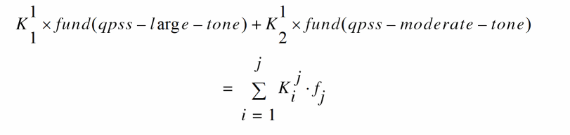
When there are L tones total in the QPSS analysis (1 large tone and L-1 moderate tones), there is also a given set of n integer vectors representing the sidebands

K¹ = { K¹₁, ..., K¹_j,..., K¹_L} K² = { K²₁, ..., K²_j,..., K²_L} … Kⁿ = { Kⁿ₁, ..., Kⁿ_j,..., Kⁿ_L}

QPSP computes the S-parameters from each virtual port to all the others. The frequency translation from one virtual port to the other is calculated using the following.

Where

f(scattered) is the frequency to which the relevant scattering parameter represents the conversion
f(incident) represents the relative frequency of a signal incident on a port
f represents the fundamental frequency used in the corresponding QPSS analysis.

Input and Output Frequencies in QPSP

For the QPSP analysis, the frequency of the input and the frequency of the response are usually different (this is an important way in which QPSP analysis differs from SP analysis).

When you analyze a down-converting mixer with a signal in the upper sideband and you sweep the RF input frequency

The most relevant harmonic for RF input is K i={1,0}
The most relevant harmonic for IF output is Ki={0,0}

Hence, you can associate

K1={1,0} with the RF port
K2={0,0} with the IF port.

The frequency translation will be the following

S₂₁ represents the transmission of the signal from the RF port with f ( incident ) = f ( RF ) to t he IF port with f ( scattering ) = f ( IF ) = f ( RF ) + Δ f ( RF to IF ) = f ( incident ) − f ( LO ).
S ₁₁ represents the reflection of the signal back to the RF port.
S12 represents the transmission from the IF port with f ( incident ) = f (IF) to the RF port with f ( scattering ) = f ( RF ) = f ( IF ) - Δ f ( RF to IF ) = f ( incident ) + f ( LO )

If the signal is in the lower sideband, then a choice of K ₁ = {-1,0} is more appropriate.

Because the QPSP computation involves inputs and outputs at frequencies that are relative to multiple harmonics, the freqaxis and sweeptype parameters behave somewhat differently in QPSP analysis than they do in both QPAC and QPXF analyses.

The sweeptype parameter controls the way the frequencies are swept.

A relative sweeptype indicates a sweep relative to the first virtual port harmonics vector
An absolute sweeptype indicates a sweep of the absolute input source frequency

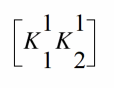
For the relative sweep with the frequenc y f _rel and th e first virtual port with harmonic vector

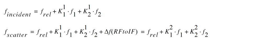
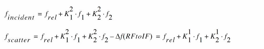
the i ncident and scatter frequencies for S21 are

while for S12 they are

For the absolute sweeptype the sweep frequency will be used as an incident frequency on the first virtual port in S₂₁

or scatter frequency for S₁₂

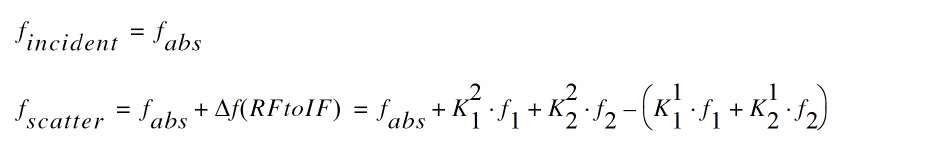
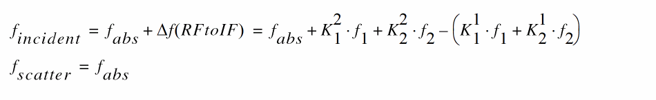
For example, with the following parameter values including relative sweeptype

QPSS fundamentals of 1000 MHz and 1010 MHz
portharmsvec = [0 1 -1 1] (to examine a down converting mixer)
sweeptype=relative
sweep range of f(rel)=0 -> 5 MHz

The frequency translation

The resulting S₂₁ represents the strength of the signal transmitted from the input at the first virtual port in the range 1010->1015 MHz to the output at the second virtual port at frequencies of 10->15 MHz. Accordingly, S₁₂ represents the signal transmitted from the second virtual port with fi_ncident=10->15 MHz to the first virtual port at f_scatter = 1010->1015 MHz.

Using the following changed parameter values including absolute sweeptype calculates the same quantities.

sweeptype=absolute
sweep range of f(abs)=1010->1015 MHz

Both configuration calculate the same quantities

f(abs) = 1010->1015 MHz

f(rel) = f(abs) - (K11*f1 + K12*f2)= 0 -> 5 MHz

because

K 1 ₁=0
K 1 ₂=1
f₁=1000 MHz
f₂=1010 MHz.

Use the freqaxis parameter to specify whether the results should be output versus the frequency at the first virtual port, the frequency at the second virtual port (out), or the absolute value of the frequency swept at the first virtual port (absin).

Requesting additional ports and harmonics increases the simulation time substantially.

Noise Analysis with QPSP

The QPSP analysis performs noise analysis which includes noise figures, equivalent noise sources, and noise parameters. The noise computation, which is performed by default and skipped only when you set donoise=no, requires additional simulation time beyond that required for S-parameter calculation.

Noise Calculations Performed by QPSP
Name	Description	Output Label
No	Total output noise at frequency f
Ns	Noise at the output due to the input probe (the source)
Nsi	Noise at the output due to the image harmonic at the source
Nso	Noise at the output due to harmonics other than input at the source
Nl	Noise at the output due to the output probe (the load)
IRN	Input referred noise	In
G	Gain of the circuit (See Note:)	Gain
F	Single sideband noise factor	F
NF	Single sideband noise figure	NF
Fdsb	Double sideband noise factor	F_dsb
NFdsb	Double sideband noise figure	NF_dsb
Fieee	IEEE single sideband noise factor	F_ieee
NFieee	IEEE single sideband noise figure	NF_ieee

For the QPSP analysis, the gain computed is the voltage gain from the actual circuit input to the circuit output, not the gain from the internal port voltage source to the output. For the noise characterization the first virtual port is dedicated as the input, the second virtual port serves as the output.

Spectre RF performs the following noise calculations.

Input referred noise

Single sideband noise factor

Single sideband noise figure

Double sideband noise factor

Double sideband noise figure

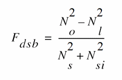
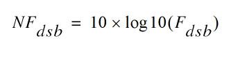
IEEE single sideband noise factor

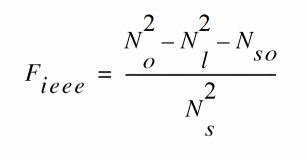
IEEE single sideband noise figure

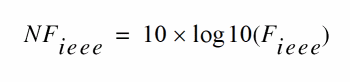
Noise Folding Effects

To ensure accurate noise calculations, set the clockmaxharm parameter to include the relevant noise folding effects.The clockmaxharm parameter is only relevant to the noise computation features of QPSP.

Swept QPSP Analysis

Specify sweep limits by providing either the end points (start and stop) or by providing the center value and the span of the sweep (center and span).

Specify sweep steps as linear or logarithmic. Either specify the number of steps or the size of each step. You can give a step-size parameter (step, lin, log, dec) to determine whether the sweep is linear or logarithmic. If you do not give a step-size parameter, the sweep is linear when the ratio of stop to start values is less than 10, and logarithmic when this ratio is 10 or greater.

Alternatively, you may specify the particular values that the sweep parameter should take using the values parameter. If you give both a specific set of values and a set of values specified using a sweep range, the two sets are merged and collated before being used. All frequencies are in Hertz.

QPSP Parameters

For information on QPSP analysis parameters, refer to the Quasi-Periodic S-Parameter Analysis (qpsp) section in the Spectre Circuit Simulator Reference manual.

Quasi-Periodic Transfer Function Analysis (QPXF)

A conventional transfer function (QPXF) analysis computes the transfer function from every source in the circuit to a single output. It differs from a conventional AC analysis in that the AC analysis computes the response from a single stimulus to every node in the circuit. The differences between the QPAC and QPXF analyses are similar. The Quasi Periodic Transfer Function or QPXF analysis computes the transfer functions from any source at any frequency to a single output at a single frequency. Thus, like QPAC analysis, QPXF analysis includes frequency conversion effects.

The QPXF analysis directly computes

Conversion Efficiency – The transfer function from the input to the output at a specified frequency.
Image Rejection and Sideband Rejection – The transfer function from the input to output at an undesired frequency.
LO Feed-Through and Power Supply Rejection – The transfer function from an undesired input to output at all frequencies.

Computing the small-signal response of a quasi-periodically varying circuit is a two step process.

First, the small stimulus is ignored and the quasi-periodic steady-state response of the circuit to possibly large periodic stimuli is computed with a QPSS analysis. As a normal part of the QPSS analysis, the quasi-periodically time-varying representation of the circuit is computed and saved for later use.
Second, the small stimulus is applied to the quasi-periodically time-varying linear representation and the small signal response is computed. This is done using the QPXF analysis.

QPXF Output Frequencies and Sideband Vectors

Either voltage or current can be the QPXF output variable of interest. The variable’s frequency is not constrained by the period of the large signal quasi-periodic solution. When you sweep a selected output frequency, you select the set of quasi-periodic small-signal input frequencies you are interested in by setting either the clockmaxharm or the sidevec output parameter.

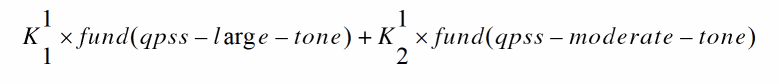
When there are L tones total in the QPSS analysis (1 large tone and L-1 moderate tones), there is also a given set of n integer vectors representing the sidebands

K¹ = { K¹₁, ..., K¹_j,..., K¹_L} K² = { K²₁, ..., K²_j,..., K²_L} … Kⁿ = { Kⁿ₁, ..., Kⁿ_j,..., Kⁿ_L}

The QPXF analysis computes the output frequency corresponding to each sideband as follows.

where

f(out) represents the (possibly swept) output signal frequency
f _j represents the fundamental frequency used in the corresponding QPSS analysis.

When you analyze a down-converting mixer, while sweeping the IF output frequency

K _i={1,0} for the RF input represents the first upper-sideband
K _i={-1,0} for the RF input represents the first lower-sideband.

Enter the sidevec parameter as a sequence of integer numbers separated by spaces. For example, you would enter the set of vectors {1 1 0} {1 -1 0} {1 1 1} as follows

sidevec=[ 1 1 0 1 -1 0 1 1 1]

The other way to specify the sidebands is the clockmaxharm parameter and the maxharms parameter in preceding QPSS analysis. Only the large tone, the first fundamental in QPSS, is affected by the QPAC clockmaxharm parameter value. It limits the maximum harmonic order of the large tone that will be considered. All the remaining tones, the moderate tones, are limited by the QPSS maxharms parameter value.

Given the following parameters

In the QPSS analysis, maxharms=[ k ⁰_max k ²_max ... k ⁿ_max]
In the QPXF analysis, clockmaxharm= K _max

The QPXF analysis output generates the following number of sidebands

(2*Kmax+1)*(2*k2max+1)*(2*k3max+1)*...*(2*knmax+1)

The number of sidebands you request substantially increases the simulation time.

For a QPXF analysis, the stimulus and response frequencies are usually different (this is an important way in which QPXF differs from XF analysis).

Use the QPXF freqaxis parameter to specify how to output the QPXF simulation results. For

freqaxis=in the results are output versus the input frequency
freqaxis=out the results are output versus the output frequency
freqaxis=absin the results are output versus the absolute value of the input frequency

You can specify the output for the QPXF analysis with either a probe component or with a pair of nodes. Any component with two or more terminals can be a voltage probe. When there are more than two terminals, the terminals are grouped in pairs and you use the portv parameter to select the appropriate pair of terminals. Alternatively, you can simply give a pair of nodes to specify a voltage as the output.

Any component that naturally computes current as an internal variable can be a current probe. If the probe component computes more than one current, use the porti parameter to select the appropriate current. Do not specify both portv and porti parameters for a simulation. If you specify neither a portv or porti parameter, the probe component provides a reasonable default.

Transfer Function Inputs

The QPXF stimuli parameter specifies the transfer function inputs. You have two choices.

The stimuli=sources parameter value uses the sources present in the circuit as inputs. You can adjust the computed gain to compensate for gains or losses in a test fixture with the xfmag parameters provided by the sources. You can use the save and nestlvl parameters to limit the number of sources in hierarchical netlists.
The stimuli=nodes_and_terminals parameter value computes all possible transfer functions. This is useful when you do not know in advance which transfer functions might be interesting.

By default, the transfer functions are computed from a small set of terminals.

If you want transfer functions from specific terminals, specify the terminals in the save statement. Use the :probe modifier (ex. Rout:1:probe) or specify useprobes=yes on the options statement.
If you want transfer functions from all terminals, specify currents=all and useprobes=yes on the options statement.

Swept QPXF Analysis

Specify sweep limits by providing either the end points (start and stop) or by providing the center value and the span of the sweep (center and span).

Specify sweep steps as linear or logarithmic as well as the number of steps or the size of each step. You can give a step-size parameter (step, lin, log, dec) to determine whether the sweep is linear or logarithmic. If you do not give a step-size parameter, the sweep is linear when the ratio of stop to start values is less than 10, and logarithmic when this ratio is 10 or greater.

Alternatively, you may specify the particular values that the sweep parameter should take using the values parameter. If you give both a specific set of values and a set specified using a sweep range, the two sets are merged and collated before being used. All frequencies are in Hertz.

QPXF Parameters

For information on QPXF analysis parameters, refer to the Quasi-Periodic Transfer Function Analysis (qpxf) section in the Spectre Circuit Simulator Reference manual.

Harmonic Balance Steady State Analysis (HB)

This analysis uses harmonic balance (in the frequency domain) to compute the response of circuits that have either one fundamental frequency (periodic steady-state, PSS) or that have multiple fundamental frequencies (quasi-periodic steady-state, QPSS). The simulation time required for an HB analysis is independent of the time-constants of the circuit. This analysis also determines the circuit’s periodic or quasi-periodic operating point, which can then be used during a periodic or quasi-periodic time-varying small-signal analysis, such as HBAC or HBnoise.

Usually, harmonic balance (HB) analysis is a very efficient way to simulate weakly nonlinear circuits. Also, HB analysis works better than shooting analysis (in the time domain) for frequency dependent components, such as delay, transmission line, and S-parameter data.

An HB analysis consists of two phases. The first phase calculates an initial solution, which the second phase then uses to compute the periodic or quasi-periodic steady-state solution, using the Newton method.

The two most important parameters for HB analysis are funds and maxharms. The funds parameter accepts a list of names of fundamentals that are present in the sources. These names are specified in the sources by the fundname parameter. When only one name appears, the analysis is an HB PSS analysis. When more than one name appears, the analysis is an HB QPSS analysis. The maxharms parameter accepts a list of numbers of the harmonics that are required to adequately model the responses due to the different fundamentals.

The annotate parameter has two values specific to HB analysis: detailed_hb and internal_hb. When annotate is set to detailed_hb or internal_hb, additional analysis debug information is printed to the log files. In the case of internal_hb, encrypted debug information is stored in the internal log file. Both options are valid for pss and qpss analyses with flexbalance=yes.

Using Multi-rate Harmonic Balance to Improve Performance

When the signals in different parts of an RF circuit have different fundamental frequencies and numbers of harmonics, it is often unnecessary and computationally costly to use a single harmonic set for all parts of the circuit. The multi-rate harmonic balance capability, by dividing the circuit into parts based on the signals contained in them, provides a way to avoid this problem.

For example, consider an RF circuit with three parts (a divider, a mixer, and an output module) and three tones (LO, RF1, and RF2).

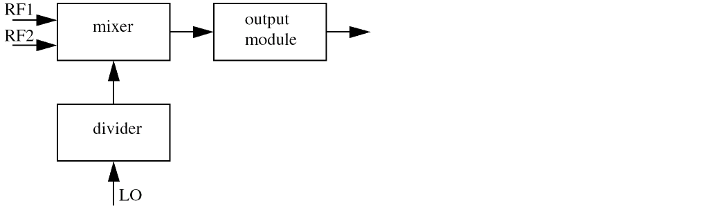
The divider has no interaction with RF1 and RF2 so the harmonic set can be [10 0 0]; the mixer interacts with all the tones so that harmonic set can be [5 3 3]; and the output module harmonic set can be [3 3 3]. If the HB engine had to use a single harmonic set, it would be [10 3 3] for all the modules, but the multi-rate harmonic balance capability allows different harmonic sets to be used for different parts of the circuit. In this example, the design can be set up to use [10, 0, 0] for the divider; [5, 3, 3] for the mixer, and [3, 3, 3] for the output.

In other words, HB multi-rate harmonic balance is a method of decomposing a circuit so that multi-rate behavior can be exploited to increase simulation performance. Of course, if every part of a circuit has the same spectrum structure (such as fundamental frequency and bandwidth), there is no need to use multi-rate harmonic balance.

Multi-rate harmonic balance is only supported for driven circuits, but will be supported for autonomous circuits at a future time.

HB Synopsis

Name ( [p] [n] ) hb <parameter=value> ...

HB Parameters

For information on harmonic balance parameters, refer to the Harmonic Balance Steady State Analysis (hb) section in the Spectre Circuit Simulator Reference manual.

Details about Using HB Analysis Parameters

The initial transient analysis provides a flexible mechanism to direct the circuit to a particular steady-state solution of interest and to avoid undesired solutions. The initial transient simulation also helps convergence by eliminating the large, but fast decaying, modes that are present in many circuits.

In some circuits, the linearity of the relationship between the initial and final states depends on when HB analysis begins. In practice, starting analysis at a good point can improve convergence, and starting at a bad point can degrade convergence and slow the analysis.

oscic Parameter

When HB analysis is used for oscillators, initialization is performed to obtain an initial guess of the steady state solution and of the oscillating frequency. Two initialization methods are implemented, based on transient and linear analysis.

When oscic=default is specified, transient initialization is used and the length of the transient is specified by tstab. You must start the oscillator using initial conditions or using a brief impulsive stimulus, just as you would if you were simulating the turn-on transient of the oscillator using transient analysis. Initial conditions would be provided for the components of the oscillator’s resonator. If an impulsive stimulus is used, it should be applied so as to couple strongly into the oscillatory mode of the circuit and poorly into any other long-lasting modes, such as those associated with bias circuitry. The Designer’s Guide to Spice and Spectre [K. S. Kundert, Kluwer Academic Publishers, 1995] describes in depth some techniques for starting oscillators.
When oscic=lin is specified, linear initialization is used. In this method, both oscillation frequency and amplitude are estimated based on linear analysis at the DC solution. No impulsive stimulus or initial conditions are needed. Linear initialization is suitable for linear oscillators such as LC and crystal oscillators. Note that tstab transient is still performed after linear initialization, though it can be significantly shortened or skipped. Either way, specifying a non-zero tstab parameter can improve convergence.

funds Parameter

For the funds parameter, the frequencies associated with fundamentals are figured out automatically by the simulator. An important feature is that each input signal can be a composition of more than one source. However, these sources must have the same fundamental name. For each fundamental name, the fundamental frequency is the greatest common factor of all frequencies associated with the name. Omitting a fundamental name in the funds parameter is an error that stops the simulation. If maxharms is not given, a warning message is issued, and the number of harmonics defaults to 1 for each of the fundamentals in a multi-tone simulation and to 10 in a single-tone simulation.

hbpartition_defs Parameter

HB signal partition is a method of decomposing a circuit so that multi-rate behavior can be exploited to increase simulation performance. If every part of a circuit has the same spectrum structure, such as fundamental frequency and bandwidth, there is no need to apply signal partition. However, if the RF circuit has multiple tones, the signals in different parts can have various spectrum structures, such as different fundamental frequency and number of harmonics. With HB signal partition, you can divide the circuit into several parts based on the signals contained in them. The parameter hbpartition_defs defines the partitions. Each partition can be made up of one or more instances. For example,

hbpartition_defs = ["I9 I10" "I11 I12" "I13 I14"]

defines three partitions. The first partition consists of instance "I9" and "I10" while the second partition consists of instances "I11" and "I12".The third one has "I13" and "I14". The number of instances for each partition should not be less than 1 and there is no upper limit for the number.

hbpartition_harms Parameter

The principle for dividing a circuit is that the subcircuits or instances with the same spectrum properties should be put into one partition. The parameter hbpartition_harms specifies the maximum number of positive harmonics of each tone for every partition. For example:

hbpartition_harms=["10 0 0" "5 3 3" "3 3 3"]

So, the maximum number of positive harmonics for the first partition is 10, 0 and 0, respectively. For the second partition, it is 5, 3 and 3. For the last one, it is 3, 3 and 3.

hbpartition_fundratios Parameter

The parameter hbpartition_fundratios indicates the fundamental frequency ratio of each tone for each partition. With these ratios, it is easy to know the fundamental frequencies of each tone of the partitions. For example:

hbpartition_fundratios=["2 1 1" "1 1 1" "1 1 1"]

If three global fundamental frequencies are defined as: LO=1GHz, RF1=1.1GHz and RF2=1.13GHz, it indicates the fundamental frequencies of each tone of the first partition is 2*LO, 1*RF1, and 1*RF2, respectively. The second and third partition has the same frequencies for their each tone: 1*LO, 1*RF1 and 1*RF2. However, you have to make sure that the global fundamental frequencies for each tone are the smallest among all the partitions and the ratios are integers.

cmin Parameter

If the circuit you are simulating can have infinitely fast transitions (for example, a circuit that contains nodes with no capacitance), the simulator might not converge well. To avoid this, you must prevent the circuit from responding instantaneously. You can accomplish this by setting cmin, the minimum capacitance to ground at each node, to a physically reasonable nonzero value. This often significantly improves convergence.

hbhomotopy Parameter

The convergence rate of large signal analyses is mainly determined by two factors: the initial condition and the nonlinearity of the circuit. When the initial condition is close to the true solution and the nonlinearity is small, convergence is typically fast. One way to calculate the initial condition is by running a transient analysis but with this method it is hard to determine how long the transient analysis needs to run.

The homotopy method uses a different approach. Given a circuit with strong nonlinearity, the homotopy method obtains a solution by starting from the same circuit but with an altered, much lower nonlinearity. Then the method increases the nonlinearity, using the solution from the lower nonlinearity as the initial condition. When the nonlinearity of the circuit reaches the original nonlinearity, a good initial condition is available from the previous solution so convergence is fast. Source stepping is used to change the nonlinearity of the circuit.

In another method, a resistor and a parallel capacitor are added between each circuit node and the ground. These components reduce the dynamic range of the circuit and help with convergence. Initially, this method obtains a solution by assuming a small resistor value. Then the method increases the resistance and obtains a new solution, using as the initial value the solution obtained on the previous iteration. When the resistance becomes large enough, the inserted components become negligible and the iteratively derived solution provides a good guess of the true solution.

The parameter used to control HB homotopy is called hbhomotopy. The parameter has the possible values source, tone (which is the default), tstab, and gsweep.

For the source value, the initial condition is generated by stepping the RF source level. This value is appropriate when the power level of the large tone or of the RF tones is high. Because there is no source available in autonomous circuits, this value is not applicable to oscillators.
For the tone value, a single tone solution is generated by turning off all the tones except the first one. The multi-tone circuit is then solved by restoring all the tones and using the single-tone solution as the initial guess. This value is appropriate for multitone designs with a strong first tone.
For the tstab value, the initial condition is generated by the usual transient analysis described above. This value is appropriate when the circuit contains devices, such as digital frequency dividers, that display strong non-linear behavior.
For the gsweep value, a resistor of conductance g is connected with each node. The conductance g is swept under the control of the gstart, gstop, and glog parameters. This value is appropriate for circuits containing high-impedance or quasi-floating nodes.

ic Parameter

You can specify the initial condition for the transient analysis by using the ic statement or the ic parameter on the capacitors and inductors. If you do not specify the initial condition, the DC solution is used as the initial condition.

If you specify an initial condition file with the readic parameter, initial conditions from the file are used, and any ic statements are ignored.

When you specify initial conditions, the simulator computes the actual initial state of the circuit by performing a DC analysis. During this analysis, the simulator forces the initial conditions on nodes by using a voltage source in series with a resistor whose resistance is rforce (see options).

With the ic statement, it is possible to specify an inconsistent initial condition (one that cannot be sustained by the reactive elements). Examples of inconsistent initial conditions include setting the voltage on a node with no path of capacitors to ground or setting the current through a branch that is not an inductor. If you initialize the simulator inconsistently, its solution jumps; that is, it changes instantly at the beginning of the simulation interval. You should avoid such changes because the simulator can have convergence problems while trying to make the jump.

Initial conditions and nodesets have similar implementations but produce different effects. Initial conditions actually define the solution, whereas nodesets only influence it. When you simulate a circuit with a transient analysis, Spectre forms and solves a set of differential equations. However, differential equations have an infinite number of solutions, and a complete set of initial conditions must be specified to identify the desired solution. Any initial conditions you do not specify are computed by the simulator to be consistent. The transient waveforms then start from initial conditions. Nodesets are usually used as a convergence aid and do not affect the final results. However, in a circuit with more than one solution, such as a latch, nodesets bias the simulator toward finding the solution closest to the nodeset values.

readns Parameter

Nodesets help the simulator find the DC or initial transient solution. You can supply nodesets in the circuit description file with nodeset statements, or in a separate file using the readns parameter. When nodesets are given, Spectre computes an initial guess of the solution by performing a DC analysis while forcing the specified values onto nodes by using a voltage source in series with a resistor whose resistance is rforce. Spectre then removes these voltage sources and resistors and computes the true solution from this initial guess.

Nodesets have two important uses. First, if a circuit has two or more solutions, nodesets can bias the simulator toward computing the desired one. Second, they are a convergence aid. By estimating the solution of the largest possible number of nodes, you might be able to eliminate a convergence problem or dramatically speed convergence.

Nodesets and initial conditions have similar implementations but produce different effects. Initial conditions actually define the solution, whereas nodesets only influence it. When you simulate a circuit with a transient analysis, Spectre forms and solves a set of differential equations. However, differential equations have an infinite number of solutions, and a complete set of initial conditions must be specified to identify the desired solution. Any initial conditions you do not specify are computed by the simulator to be consistent. The transient waveforms then start from initial conditions. Nodesets are usually used as a convergence aid and do not affect the final results. However, in a circuit with more than one solution, such as a latch, nodesets bias the simulator toward finding the solution closest to the nodeset values.

skipdc Parameter

You can skip the DC analysis entirely by using the skipdc parameter. If the DC analysis is skipped, the initial solution will be either trivial or given in the file you specified by the readic parameter, or, if the readic parameter is not given, the values specified on the ic statements. Device-based initial conditions are not used for skipdc. Nodes that you do not specify with the ic file or ic statements start at zero. You should not use this parameter unless you are generating a nodeset file for circuits that have trouble in the DC solution; it usually takes longer to follow the initial transient spikes that occur when the DC analysis is skipped than it takes to find the real DC solution. The skipdc parameter might also cause convergence problems in the transient analysis.

Harmonic Balance AC Analysis (HBAC)

The harmonic balance AC (HBAC) analysis computes transfer functions for circuits that exhibit single or multi-tone frequency translation. Such circuits include mixers, switched-capacitor filters, samplers, phase-locked loops, and the like. HBAC is a small-signal analysis like AC analysis, except the circuit is first linearized about a periodically or quasi-periodically varying operating point rather than about a simple DC operating point. Linearizing about a periodically or quasi-periodically time-varying operating point allows transfer-functions that include frequency translation, whereas simply linearizing about a DC operating point cannot because linear time-invariant circuits do not exhibit frequency translation. Also, the frequency of the sinusoidal stimulus is not constrained by the period of the large periodic solution.

Computing the small-signal response of a periodically or quasi-periodically varying circuit is a two step process. First, the small stimulus is ignored and the periodic or quasi-periodic steady-state response of the circuit to possibly large periodic stimuli is computed using HB analysis. As a normal part of the HB analysis, the periodically or quasi-periodically time-varying representation of the circuit is computed and saved for later use. Second, the small stimulus is applied to the periodically varying linear representation to compute the small signal response. This is done using the HBAC analysis. A HBAC analysis cannot be used alone, it must follow a HB analysis. However, any number of periodic or quasi-periodic small-signal analyses, such as HBAC or HBnoise, can follow a HB analysis.

Modulated small signal measurements are possible using the Analog Design Environment (ADE). The modulated option for HBAC and other modulated parameters are set by ADE. HBAC analyses with this option produce results that can have limited use outside of ADE. Direct Plot is configured to analyze these results and combine several wave forms to measure AM and PM response due to single sideband or modulated stimuli. For details, see the Spectre Circuit Simulator and Accelerated Parallel Simulator RF Analysis in ADE Explorer User Guide.

Unlike other analyses in Spectre, the HBAC analysis can sweep only frequency.

HBAC Synopsis

Name hbac <parameter=value> ...

HBAC Parameters

For information on hbac analysis parameters, refer to the HB AC Analysis (hbac) section in the Spectre Circuit Simulator Reference manual.

Details about Using HBAC Analysis Parameters

freqaxis Parameter

With HBAC, the frequency of the stimulus and of the response are usually different—this is one important way that HBAC differs from AC. The freqaxis parameter is used to specify whether the results should be output versus the input frequency (in), the output frequency (out), or the absolute value of the output frequency (absout).

maxsideband and sidevec Parameters

You can select the set of periodic small-signal output frequencies of interest by setting either the maxsideband or the sidevec parameters.

When there is only one tone in HB analysis, sidebands are n integer numbers, K1, K2, ..., Kn, and the output frequency at each sideband is computed as

f(out)= f(in) + Ki * fund(hb)

where f(in) represents the (possibly swept) input frequency, and fund(hb) represents the fundamental frequency used in the corresponding HB analysis. Thus, when analyzing a down-converting mixer, while sweeping the RF input frequency, the most relevant sideband for IF output is Ki= -1. When simulating an up-converting mixer, while sweeping IF input frequency, the most relevant sideband for RF output is Ki= 1. By setting the maxsideband value to Kmax, all 2 * Kmax + 1 sidebands from -Kmax to +Kmax are generated.

When there are multiple tones in HB analysis, sidebands are vectors. Assume we have one large tone and one moderate tone in HB. A sideband, K1, is represented as [K1_1 K1_2]. The corresponding frequency is

K1_1 * fund(large tone of HB) + K1_2 * fund(moderate tone of HB)

We assume that there are L large and moderate tones in HB analysis and a given set of n integer vectors representing the sidebands, K1 = { K1_1, ..., K1_j, ..., K1_L}, K2, ..., Kn. The output frequency at each sideband is computed as

f(out)= f(in) + SUM_j=1_to_L{Ki_j * fund_j(hb)}

where f(in) represents the (possibly swept) input frequency, and fund_j(hb) represents the fundamental frequency used in the corresponding HB analysis. Thus, when analyzing a down-converting mixer, while sweeping the RF input frequency, the most relevant sideband for IF output is {-1, 0}. When simulating an up-converting mixer, while sweeping IF input frequency, the most relevant sideband for RF output is {1, 0}. You enter sidevec as a sequence of integer numbers, separated by spaces. The set of vectors {1 1 0} {1 -1 0} {1 1 1} becomes sidevec=[1 1 0 1 -1 0 1 1 1]. For maxsideband, only the large tone, the first fundamental, is affected by this entry. All the other tones, the moderate tones, are limited by maxharms, specified for a HB analysis. Given maxharms=[k1max k2max ... knmax] in HB and maxsideband=Kmax, all

(2*Kmax + 1)*(2*k2max+1)*(2*k3max+1) *...*(2*knmax+1)

sidebands are generated.

The number of requested sidebands has a significant impact on the simulation time.

Sweep Interval Parameters

Harmonic Balance Noise Analysis (HBnoise)

The harmonic balance periodic or quasi-periodic noise (HBnoise) analysis is similar to conventional noise analysis, except that HBnoise analysis includes frequency conversion effects. As a consequence, it is useful for predicting the noise behavior of mixers, switched-capacitor filters, and other periodically driven circuits. It is particularly useful for predicting the phase noise of autonomous circuits, such as oscillators.

HBnoise analysis linearizes the circuit about the periodic or quasi-periodic operating point computed in the prerequisite HB analysis. It is the periodically or quasi-periodically time-varying nature of the linearized circuit that accounts for the frequency conversion. In addition, the effect of a periodically or quasi-periodically time-varying bias point on the noise generated by the various components in the circuit is also included.

The time-average of the noise at the output of the circuit is computed in the form of a spectral density versus frequency. The output of the circuit is specified with either a pair of nodes or a probe component. To specify the output of a circuit with a probe, specify it using the oprobe parameter. If the output is voltage (or potential), choose a resistor or a port as the output probe. If the output is current (or flow), choose a vsource or iprobe as the output probe.

The noise analysis always computes the total noise at the output, including contributions from the input source and the output load. The amount of the output noise that is attributable to each noise source in the circuit is also computed and output individually. If the input source is identified (using iprobe) and is a vsource or isource, the input-referred noise, which includes the noise from the input source itself, is computed. Finally, if the input source is identified (using iprobe) and is noisy, as is the case with ports, the noise factor and noise figure are computed. Thus if

No = total output noise
Ns = noise at the output due to the input probe (the source)
Nsi = noise at the output due to the image harmonic at the source
Nso = noise at the output due to harmonics other than input at the source
Nl = noise at the output due to the output probe (the load)
IRN = input referred noise
G = gain of the circuit
F = noise factor
NF = noise figure
Fdsb = double sideband noise factor
NFdsb = double sideband noise figure
Fieee = IEEE single sideband noise factor
NFieee = IEEE single sideband noise figure

then,

IRN = sqrt(No^2/G^2)
F = (No^2 - Nl^2)/Ns^2
NF = 10*log10(F)
Fdsb = (No^2 - Nl^2)/(Ns^2+Nsi^2)
NFdsb = 10*log10(Fdsb)
Fieee = (No^2 - Nl^2 - Nso^2)/Ns^2
NFieee = 10*log10(Fieee)

When the results are output, No is named out, IRN is named in, G is named gain, F, NF, Fdsb, NFdsb, Fieee, and NFieee are named F, NF, Fdsb, NFdsb, Fieee, and NFieee respectively.

The computation of gain and IRN for quasi-periodic noise in HBnoise assumes that the circuit under test is impedance-matched to the input source. This can introduce inaccuracy into the gain and IRN computation.

An HBnoise analysis must follow an HB analysis.

Unlike other analyses in Spectre, this analysis can only sweep frequency.

HBnoise Synopsis

Name ( [p] [n] ... ) hbnoise <parameter=value> ...

The optional terminals (p and n) specify the output of the circuit. If you do not give the terminals, then you must specify the output with a probe component.

HBnoise Parameters

For information on hbnoise parameters, refer to the HB Noise Analysis (hbnoise) section in the Spectre Circuit Simulator Reference manual.

Details about Using HBnoise Analysis Parameters

iprobe Parameter

If you want the input-referred noise or noise figure, specify the input source using the iprobe parameter. For input-referred noise, use either a vsource or isource as the input probe; for noise figure, use a port as the probe. Currently, only a vsource, an isource, or a port can be used as an input probe. If the input source is noisy, as is a port, the noise analysis computes the noise factor (F) and noise figure (NF). To match the IEEE definition of noise figure, the input probe must be a port with no excess noise and its noisetemp must be set to 16.85C (290K). In addition, the output load must be a resistor or port and must be identified as the oprobe.

If port is specified as the input probe, then both input-referred noise and gain are referred back to the equivalent voltage source inside the port. S-parameter analysis calculates those values.

maxsideband Parameter

In practice, noise can mix with each of the harmonics of the periodic drive signal applied in the HB analysis and end up at the output frequency. However, the HBnoise analysis only includes the noise that mixes with a finite set of harmonics that are typically specified using the maxsideband parameter.

If Ki represents sideband i, then for periodic noise,

f(noise_source) = f(out) + Ki * fund(hb)

For quasi-periodic noise with multiple tones in HB analysis, assuming there are one large tone and one moderate tone, Ki is represented as [Ki_1 Ki_2]. The corresponding frequency shift is

Ki_1 * fund(large tone of HB) + Ki_2 * fund(moderate tone of HB)

Assuming that there are L large and moderate tones in HB analysis and a set of n integer vectors representing the sidebands

K1 = { K1_1,...K1_j..., K1_L}, K2, ..., Kn.

Then

f(noise_source) = f(out) +  SUM_j=1_to_L{ Ki_j * fund_j(hb) }

The maxsideband parameter specifies the maximum |Ki| included in the HBnoise calculation. For quasi-periodic noise, only the large tone, the first fundamental, is affected by this entry. All the other tones, the moderate tones, are limited by maxharms, specified for a HB analysis.

The number of requested sidebands changes the simulation time substantially.

When HBnoise analysis does only an xf analysis (xfonly=yes), the variable of interest at the output can be voltage or current, and its frequency is not constrained by the period of the large periodic solution. While sweeping the selected output frequency, you can select the periodic small-signal input frequencies of interest by setting the maxsideband parameter. With this analysis, the frequency of the stimulus and of the response are usually different (this is an important way that this analysis differs from XF).

refsideband Parameter

The reference sideband (refsideband) specifies which conversion gain is used when computing input-referred noise, noise factor, and noise figure. The reference sideband specifies the input frequency relative to the output frequency with:

|f(input)| = |f(out) + refsideband frequency shift|

For periodic noise (only one tone in HB analysis), the refsideband is a number. Use refsideband=0 when the input and output of the circuit are at the same frequency (such as with amplifiers and filters). When refsideband differs from 0, the single side-band noise figure is computed.

While for quasi-periodic noise (multiple tones in HB analysis), reference sidebands are vectors. Assume we have one large tone and one moderate tone in HB. A sideband Ki will be a vector [Ki_1 Ki_2]. It gives the frequency at

Ki_1 * fund(large tone of HB) + Ki_2 * fund(moderate tone of HB)

Use refsideband=[0 0 ...] when the input and output of the circuit are at the same frequency (such as with amplifiers and filters).

stimuli Parameter

You can use the stimuli parameter to specify what serves as the inputs for the transfer functions.

stimuli=sources indicates that the sources present in the circuit are to be used. You can use the xfmag parameters provided by the sources to adjust the computed gain to compensate for gains or losses in a test fixture. You can limit the number of sources in hierarchical netlists by using the save and nestlvl parameters.
stimuli=nodes_and_terminals indicates that all possible transfer functions are to be computed. This is useful when you do not know in advance which transfer functions are interesting. Transfer functions for nodes are computed assuming that a unit magnitude flow (current) source is connected from the node to ground. Transfer functions for terminals are computed assuming that a unit magnitude value (voltage) source is connected in series with the terminal. By default, the transfer functions from a small set of terminals are computed. If you want transfer functions from specific terminals, specify the terminals in the save statement. You must use the :probe modifier (for example, Rout:1:probe) or specify useprobes=yes on the options statement. If you want transfer functions from all terminals, specify currents=all and useprobes=yes on the options statement.

With HBnoise analysis, transfer function outputs are always available.

Sweep Interval Parameters

xfonly Parameter

When option xfonly is set to yes, HBnoise analysis does only a conventional transfer function (xf) analysis, which computes the transfer function from every source in the circuit to a single output. This analysis differs from a conventional AC analysis in that the AC analysis computes the response from a single stimulus to every node in the circuit. HBnoise computes the transfer functions from any source at any frequency to a single output at a single frequency. Thus, like HBAC analysis, it includes frequency conversion effects. It directly computes such useful quantities as conversion efficiency (transfer function from input to output at desired frequency), image and sideband rejection (input to output at undesired frequency), and LO feed-through and power supply rejection (undesired input to output at all frequencies).

HB S-Parameter Analysis (hbsp)

The periodic or quasi-periodic SP (HBSP) analysis is used to compute scattering and noise parameters for n-port circuits such as mixers that exhibit frequency translation. It is a small-signal analysis similar to SP analysis, except that in HBAC and HBNOISE, the circuit is first linearized about a periodically varying operating point as opposed to a simple DC operating point. Linearizing about a periodically or quasi-periodically time-varying operating point allows the computation of S-parameters between circuit ports that convert signals from one frequency band to another. HBSP can also calculate noise parameters in frequency-converting circuits. In addition, HBSP computes noise figure (both single-sideband and double-sideband), input referred noise, equivalent noise parameters, and noise correlation matrices. Similar to HBNOISE, but unlike SP, the noise features of the HBSP analysis include noise folding effects due to the periodic time-varying nature of the circuit.

Computing the n-port S-parameters and noise parameters of a periodically varying circuit is a two-step process. First, the small stimulus is ignored and the periodic or quasi-periodic steady-state response of the circuit to possibly large periodic stimulus is computed using HB analysis. As a part of the HB analysis, the periodically time-varying representation of the circuit is computed and saved for later use. The second step is applying small-signal excitations to compute the n-port S-parameters and noise parameters. This is done using the HBSP analysis. HBSP analysis cannot be used independently; it must follow HB analysis. However, any number of periodic small-signal analyses such as HBAC, HBSP, HBNOISE, can follow an HB analysis.

Unlike other analyses in Spectre, this analysis can only sweep frequency.

HBSP Parameters

For information on hbsp analysis parameters, refer to the HB S-Parameter Analysis (hbsp) section in the Spectre Circuit Simulator Reference manual.

To specify the HBSP analysis, the port and port harmonic relations must be specified. You can select the ports of interest by setting the port parameter, and select the set of periodic small-signal output frequencies of interest by setting portharmsvec or harmsvec parameters. For a given set of n integer numbers representing the harmonics K1, K2, ... Kn, the scattering parameters at each port are computed at the following frequencies:

For periodic SP in one-tone HB analysis, frequency is:

f(scattered)= f(rel) + Ki * fund(HB)

For quasi-periodic noise with multi-tone in HB analysis, sidebands are vectors. Consider that you have one large tone and one moderate tone in HB. Then, the above sideband K1 will be represented as [K1_1 K1_2]. In this case, the corresponding frequency is:

K1_1 * fund(large tone of HB) + K1_2 * fund(moderate tone of HB)= SUM_j=1_to_L{Ki_j * fund_j(HB)}

If there are L (1 large and L-1 moderate) tones in HB analysis and a given set of n integer vectors representing the sidebands:

K1 = { K1_1,...K1_j..., K1_L } , K2, ... Kn

If you specify the relative frequency, the scattering parameters at each port are computed at the frequencies:

f(scattered)= f(rel) + SUM_j=1_to_L{Ki_j * fund_j(hb)},

where f(rel) represents the relative frequency of a signal incident on a port, f(scattered) represents the frequency to which the relevant scattering parameter represents the conversion, and fund(one-tone HB) or fund_j(multi-tone HB) represents the fundamental frequency used in the corresponding HB analysis.

During analysis of a down-converting mixer with a blocker and the signal in the upper sideband, we sweep the input frequency of the signal coming into RF port. In case of periodic SP with one-tone HB, the most relevant harmonic for RF input is Ki= 1 and for IF output Ki= 0. Therefore, we can associate K2=0 with the IF port and K1=1 with the RF port. S21 represents the transmission of signal from the RF to IF, and S11 represents the reflection of signal back to the RF port. If the signal was in the lower sideband, a choice of K1=-1 is more appropriate. For quasi-periodic SP with multi-tone HB, the most relevant sideband for this input is Ki= {1 , 0} and for IF output Ki= {0 , 0}. Therefore, we can associate K1={1 , 0} with the RF port and K2={0 , 0} with the IF port. If the signal was in the lower sideband, then a choice of K1={-1 , 0} is more appropriate.

portharmsvec or harmsvec parameters can be used to specify the harmonics of interest. If portharmsvec is specified, the harmonics must be in one-to-one correspondence with the ports, with each harmonic associated with a single port. If harmonics are specified in the optional harmsvec parameter, all possible frequency-translating scattering parameters associated with the specified harmonics are computed.

With HBSP the frequency of the input and of the response are usually different (this is an important area in which HBSP differs from SP). Because the HBSP computation involves inputs and outputs at frequencies that are relative to multiple harmonics or sidebands, the freqaxis and sweeptype parameters behave differently in HPSP than in HBAC and HBNOISE.

The sweeptype parameter controls the way the frequencies in the HBSP analysis are swept. Specifying a relative sweep indicates the sweep to be relative to the analysis harmonics or port sideband (not the HB fundamental) and specifying an absolute sweep indicates the sweep of the absolute input source frequency.

For example, in case of periodic SP with one-tone HB and HB fundamental of 100MHz, portharmsvec set to [9 1] to examine a downconverting mixer, sweeptype=relative, and a sweep range of f(rel)=0->50MHz, S21 represents the strength of signal transmitted from the input port in the range 900->950MHz to the output port at frequencies 100->150MHz. Using sweeptype=absolute and sweeping the frequency from 900->950MHz would calculate the same quantities, because f(abs)=900->950MHz, f(rel) = f(abs) - K1 * fund(hb) = 0->50MHz, and K1=9 and fund(hb) = 100MHz.

For quasi-periodic noise with multi-tone HB, and HB fundamentals of 1000MHz (LO) and 966MHz (blocker in RF channel), portharmsvec could be set to [0 1 -1 1] to examine a downconverting mixer. Consider setting sweeptype=relative and a sweep range of f(rel)=-10MHz<->10MHz. Then, S21 will represent the strength of the signal transmitted from the input port in the range 956->976MHz to the output port at frequencies 24<->44MHz. Using sweeptype=absolute and sweeping the frequency from 966<->976MHz will calculate the same quantities, because f(abs)=956<->976MHz, f(rel) = f(abs) - ( K1_1 * fund_1(hb) + K1_2 * fund_2(hb) = -10MHz<->10MHz, andK1_1=0, K1_2=1 and fund_1(hb) = 1000MHz, fund_2(hb) = 966MHz.

The freqaxis parameter is used to specify whether the results should be output versus the scattered frequency at the input port (in), the scattered frequency at the output port (out), or the absolute value of the frequency swept at the input port (absin).

HBSP analysis also computes noise figures, equivalent noise sources, and noise parameters. The noise computation, which is skipped only when donoise=no, requires additional simulation time. If:

No = total output noise at frequency f

Ns = noise at the output due to the input probe (the source)

Nsi = noise at the output due to the image harmonic at the source

Nso = noise at the output due to harmonics other than input at the source

Nl = noise at the output due to the output probe (the load)

IRN = input referred noise

G = gain of the circuit

F = noise factor (single side band)

NF = noise figure (single side band)

Fdsb = double sideband noise factor

NFdsb = double sideband noise figure

Fieee = IEEE single sideband noise factor

NFieee = IEEE single sideband noise figure

Then:

IRN = sqrt(No^2/G^2)

F = (No^2 - Nl^2)/Ns^2

NF = 10*log10(F)

Fdsb = (No^2 - Nl^2)/(Ns^2+Nsi^2)

NFdsb = 10*log10(Fdsb)

Fieee = (No^2 - Nl^2 - Nso^2)/Ns^2

NFieee = 10*log10(Fieee).

When the results are output, IRN is named in, G is named gain, F, NF, Fdsb, NFdsb, Fieee, and NFieee are named F, NF, Fdsb, NFdsb, Fieee, and NFieee, respectively. Note that the gain computed by HBSP is the voltage gain from the actual circuit input to the circuit output, not the gain from the internal port voltage source to the output.

To ensure accurate noise calculations, the maxsideband or sidebands parameters must be set to include the relevant noise folding effects.maxsideband is only relevant to the noise computation features of HBSP.

You can specify sweep limits by giving the end points or by providing the center value and span of the sweep. Steps can be linear or logarithmic, and you can specify the number of steps or the size of each step. In addition, you can specify a step size parameter (step, lin, log, dec) to determine whether the sweep is linear or logarithmic. If you do not give a step size parameter, the sweep is linear when the ratio of stop to start values is less than 10, and logarithmic when this ratio is 10 or greater. Alternatively, you use the values parameter to specify the values that the sweep parameter should take. If you use both a specific set of values and a set specified using a sweep range, the two sets are merged and collated before being used. All frequencies are in Hertz.

Envelope Analysis (ENVLP)

Efficient and accurate prediction of the envelope transient response of RF circuits is important for RF circuit designers who are simulating communications systems. You can apply ENVLP analysis to efficiently and accurately analyze modulation signals in large communication circuits. Important applications include

Predicting the spectral regrowth of amplifiers and mixers
Designing feedback loops such as Automatic Gain Control (AGC) loops
Predicting the transient behavior of switched capacitor filters
Simulating large transients in phase lock loops
Helping the oscillator designer identify the load pull effect for the communication systems with VCO and power amplifier.

It is important to know that ENVLP Analysis is not designed to simulate circuits having a filter with nodes that have higher frequencies than clock. A transient analysis is faster for these circuits.

Modulation Signals

Many RF circuits process narrowband signals in the form of modulated carriers. Modulated carriers are characterized as having both a periodic high-frequency carrier signal and a low-frequency modulation signal. The modulation signal acts on either the amplitude, phase, or frequency of the carrier. In general, the modulation is arbitrary. The ratio between the lowest frequency in the modulation and the frequency of the carrier is a measure of the relative frequency resolution required of the simulation. Traditional transient analysis is inefficient for the resolution of low modulation frequencies in the presence of a high carrier frequency because the high-frequency carrier forces a small time step while the low-frequency modulation forces a long simulation interval.

A Mixer Example

As a typical example, a designer might be interested in simulating a receiver transmit path involving a modulator, in particular, to predict the spectral regrowth of the modulator. As shown in Figure 2-10, the inputs to a modulator can be one complete digital low-frequency (not necessarily periodic) modulation and one high frequency LO. The result is a modulated high-frequency signal as shown in Figure 2-10. However, due to the nonlinearity of the modulator, unwanted harmonics might be generated and, to validate the design, it is important to predict the signal level at these unwanted harmonics.

Figure 2-10 Time-Domain Modulation

Figure 2-11 shows a typical scenario in the receiver signal path. Due to the nonlinearity of the mixer, it is important to predict the resulting spectral regrowth. Spectral regrowth is expensive to simulate using traditional transient analysis because spectral regrowth requires a very long time interval to resolve the required frequency resolution.

Figure 2-11 Spectrum-Domain Modulation

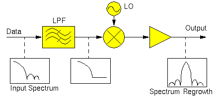
ENVLP analysis overcomes this difficulty with traditional transient analysis. ENVLP analysis reduces simulation time without compromising accuracy by exploiting the property that the behavior of a circuit in a given high frequency clock cycle is similar, but not identical, to its behavior in the preceding and following cycles. In particular, the envelope of the high-frequency clock can be followed by accurately computing the circuit behavior over occasional cycles, which accurately capture the fast transient behavior. The slow varying modulation is accurately followed by a smooth curve. As a result, the spectrum of the circuit response can be obtained by combining the spectrum of the smooth curve and the spectrum of occasional clock cycles.

RF analyses such as PSS (periodic steady-state analysis) [1] or QPSS (quasi-periodic steady-state analysis) [2] might not work directly because the modulation signal might be neither periodic nor quasi-periodic.

The clock is referred to differently in different applications.

For mixers, the clock is called the LO
For detectors, the clock is called the carrier
For switched-capacitor filters, the clock is called the clock

The clock is normally the most rapidly changing signal in the circuit and thus causes the most nonlinearity.

The Time Domain and Harmonic Balance ENVLP Algorithms

The Spectre RF ENVLP analysis uses a multi-stage multi-past-point integration algorithm that is an extension to a method introduced by Petzold [3] and further explored by Kundert, White and Sangiovanni-Vincentelli [4]. The method approximates the sample envelope as a piecewise polynomial in a manner that is analogous to conventional transient analysis. The ENVLP algorithm is based on two schemes:

Time domain shooting
Harmonic balance

In time domain shooting, the clock nonlinearity is resolved by time-domain integration. In harmonic balance, the clock nonlinearity is expressed as harmonics of fundamental frequencies.

Most RF circuits used in communication systems are clocked at a high frequency. The clock (such as LO) usually causes the most nonlinearity in the circuit response. Time-domain integration is a more efficient and accurate method of resolving strong nonlinear circuits with sharp transitions and transient details, while harmonic balance is more efficient for linear and nearly linear circuits. ENVLP analysis samples the circuit waveforms at the clock frequency, and assumes the resulting envelope can be accurately represented by a piecewise polynomial. The nonlinearity caused by the clock signal is resolved by occasional integrations of a period of circuit responses.

Time Domain Envelope (TD ENVLP) Analysis

Most circuits can be described by a system of differential equations of the form shown in Equation 2-1.

(2-1)

where

u ( t )∈ ℜ M is the vector of input sources
v ( t )∈ ℜ N (the state) is the node voltages
q(v ( t ))∈ ℜ N is the vector of node charges and fluxes
i(v ( t ))∈ ℜ N is the vector of resistive node currents

If the state v is known at some time t ₀, it is possible to solve Equation 2-1 and compute the state at some later time t ₁. In general, you can write Equation 2-2.

(2-2)

where φ : ℜ N X ℜ N X ℜ N → ℜ N is a state transition function for the differential equation.

Consider that the circuit to be simulated has an input clock with a known period T that is much smaller than the simulation interval. Assume the sequence formed by sampling the state at the beginning of each clock cycle, v (0), v ( T ), v ( 2T ), ..., v ( mT ), ..., changes slowly as a function of m, the clock cycle number. A smooth continuous function can be defined to interpolate the sequence formed by sampling the state at every time interval T .

The waveform shown in Figure 2-12, is sampled at the clock period, resulting in a circuit envelope that reveals the slow varying modulation.

Figure 2-12 A Sample Envelope

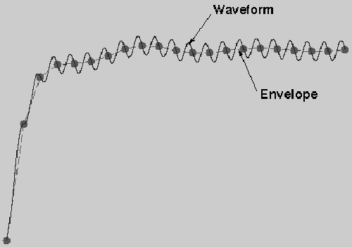
Figure 2-13 illustrates how the TD ENVLP (time domain envelope) algorithm works.

Figure 2-13 TD ENVLP Integration

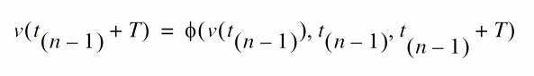
TD ENVLP integration is similar to transient integration. In this example, two past stages are used to compute a new stage. Assume the state values are known at t ₍ n _-1₎ and t ₍_n₎, which are a number of clock cycles apart from each other, and are at the beginning of the clock cycle. The state values at t ₍_n_-1₎ and t ₍_n_-1₎+ T are related by integration of one clock cycle, that is,

(2-3)

where φ is the state transition function.

Likewise, the states at t _n and t _n+ T are related by v ( t _n+ T) = φ( v ( t _n), t _n, t _n+ T ). The job of the algorithm is to find the state value at a new time point t ₍_n₊₁₎ many cycles from t _n, such that the pair v ( t _n_{+ 1}), t ₍_n_{+ 1}₎ interpolates a quadratic polynomial defined by the three state values
v ( t ₍_n_{- 1}₎), v ( t _n) and v ( t ₍_n_{+ 1}₎+ T ) at t ₍_n_{- 1}_), t _n and t ₍_n_{+ 1}₎+ T, respectively.

On one hand, the state value v ( t ₍_n_{+ 1}₎+ T ) is given by

(2-4)

On the other hand, from the interpolation condition, v ( t ₍_{n + 1}₎+ T ) can be written as a linear combination of v ( t ₍_n_{- 1}₎), v ( t _n) and v ( t _n_{+ 1}), i.e., there exist scalars α₁, α₂ and α₃ such that

(2-5)

The scalars α₁, α₂ and α₃ can be obtained by standard techniques such as by first defining a quadratic function using three state values and then asking the fourth value to be interpolated by the quadratic function. Combining the two equations gives

(2-6)

which can be used to solve for v ( t _n₊₁) by shooting Newton method.

After v ( t _n+1) is obtained, we use t _n and t ₍_n₊₁₎ as past points and solve for a new stage v ( t _n₊₂). The two-past-point one-new-stage process is repeated until the desired stop time is reached.

Harmonic Balance Envelope (HB ENVLP) Analysis

A general signal in a modulation system has the form

(2-7)

when the Fourier coefficients

are taken to be slowly varying transient waveforms.

must vary slowly relative to f k , because when the bandwidth of

is greater than f k /2, the sidebands of adjacent harmonics begin to overlap and the representation is not unique. If there is an f 0 that satisfies

(2-8)

then x(t) is a one tone signal and the corresponding analysis is a single carrier HB envelope. Otherwise, x(t) is a multi-tone signal and the corresponding analysis is a multi-carrier HB envelope.

Rewriting Equation 1-1 in the form of Equation 2-7 results in the following.

(2-9)

In vector form, this can be written as

(2-10)

where Ω is a diagonal matrix with j 2 πf_k on the k th diagonal. As the transient analysis does, an HB ENVLP analysis discretizes

with a finite-difference approximation such as the backward-Euler, trapezoidal, or Gear method. For example, applying backward-Euler, Equation 2-9 becomes

(2-11)

Equation 2-11 is a system of nonlinear algebraic equations.

can be solved by Newton's method. After that value is obtained, it is used to get

until the desired stop time is reached.

HB ENVLP analysis samples the modulation envelope in time and outputs a time-varying spectrum for time point t ₁, t ₂, ..., t _n, .... The spectrum is converted to time domain waveforms in each clock cycle.

In the first several clock cycles, a transient analysis is used in single carrier HB Envelope, as it is in TD Envelope. For multi-carrier HB Envelope, HB QPSS is adopted to get the steady state at the beginning.Then the time domain data is converted to frequency domain and Equation 2-11 works. HB Envelope is like a special Transient for frequency data.

Figure 2-14 HB Envelope Analysis outputs a time-varying spectrum

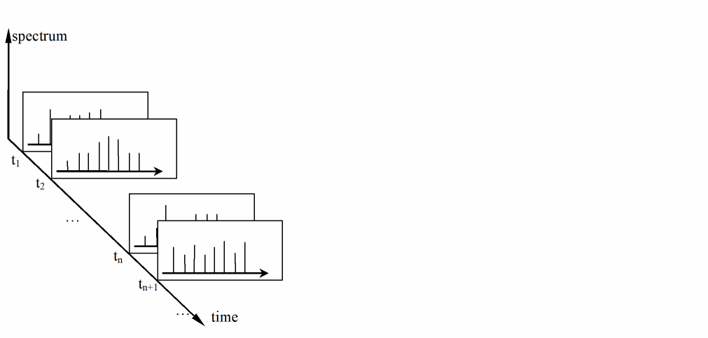
For linear and nearly linear circuits, HB Envelope is more efficient than TD Envelope analysis.

Both TD and HB Envelope analysis use Newton’s method. In a manner similar to that used for Periodic Steady-State (PSS) analysis (for details see [1]), the Newton equation is solved efficiently by a matrix-implicit iterative method. Compared to harmonic balance-based envelope following algorithms, the Spectre RF Envelope Following algorithm has advantages and weaknesses similar to Spectre RF PSS analysis versus analogous harmonic balance-based steady-state computation approaches.

In TD and single carrier HB Envelope analysis, the clock is pointed directly. In multi-carrier HB Envelope analysis, the first one of the fundamentals is regarded as the clock. The period of the clock is the time unit of the envelope analyses.

Both TD and HB Envelope analysis attempt to skip as many clock cycles as possible to achieve a faster speed than Transient analysis. Similar to Transient analysis, after a sample point is computed, it is necessary to check that the trajectory is following the low-order polynomial as assumed. If it is not, the point is discarded and the time step is reduced. If rapid changes in the envelope are encountered, Envelope analysis reduces its step size down to the point where no cycles are skipped. In this case, both TD Envelope analysis and single carrier HB Envelope analysis degenerate to a simple Transient analysis. The frequency domain data are converted to time domain. After the simple Transient, the data are converted back to frequency domain.

Generally, HB Envelope is faster than TD Envelope for linear or weakly non-linear circuits. However, HB Envelope suffers from accuracy problems when dealing with strongly non-linear circuits.

HB Parameters

Parameters required by the HB ENVLP analysis are:

Basic Parameters for HB ENVLP Analysis

`flexbalance=yes`	The HB engine shares this analysis form with the TD engine. Use the HB engine by setting `flexbalance=yes` in the analysis statement. The default is `no`.
`harms`or `maxharms`	Use of the `harms` or `maxharms` parameter is similar to the usage in driven HB analysis. For more information, see Basic HB Parameters for Driven HB Analysis table.

Optional Parameters for HB ENVLP Analysis

oversamplefactor

Use of the oversamplefactor parameter is similar to its usage in driven HB analysis. For more information, see Optional HB Parameters for Driven HB Analysis table.

Using ENVLP Analysis

This analysis computes the envelope response of a circuit. The user specifies the analysis clockname. The simulator automatically determines the clock period by looking through all the sources with the specified name. The envelope response is computed over the interval from start to stop. If the interval is not a multiple of the clock period, it is rounded off to the nearest multiple before the stop time. The initial condition is taken to be the DC steady-state solution or determined by tstab if not otherwise given. If flexbalance is yes, HB ENVLP will be used, otherwise TD ENVLP will be used. The default value is no.

As discussed previously, the clock might be referred to differently in different applications LO with mixers, carrier with detectors, and clock with switched-capacitor filters. The clock is normally the most rapidly changing signal in the circuit and thus causes the most nonlinearity.

ENVLP analysis is most efficient for circuits where the modulation bandwidth is orders of magnitude lower than the clock frequency. This is typically the case in RF circuits. Passing a narrowband signal through a nonlinear RF circuit results in a broadband signal whose spectrum is relatively sparse, as shown in Figure 2-15. The spectrum shows that due to nonlinearity, narrowband responses centered at the carrier harmonics are generated.

Figure 2-15 Spectrum of a Narrowband Signal

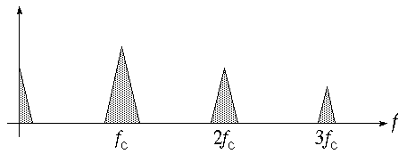
In general, this spectrum consists of clusters of frequencies near the harmonics of the carrier. When the modulation is periodic or quasi-periodic, these clusters take the form of a discrete set of frequencies. Otherwise they form a continuous distribution of frequencies.

Figures 2-16 and 2-17 present examples of calculating spectrum regrowth. Here the carrier is a periodic high-frequency signal, while the modulation is a low frequency arbitrary digital modulation. ENVLP analysis is used to accurately calculate the sparse spectrums centered at clock harmonics. A continuous spectrum in each cluster is expected because the modulation is neither periodic nor quasi-periodic.

In two typical situations, ENVLP analysis is very efficient and effective in simulating the transient behavior of circuits driven by two periodic signals.

In the first situation, one fundamental frequency is much higher than the other one, as would be the case for an up-conversion mixer. As shown in Figure 2-16, you can interpret a quasiperiodic signal with two widely separated fundamentals as a periodically modulated periodic signal. To do this, designate the high frequency signal as the carrier and the low frequency signal as the modulation. If the carrier is much higher in frequency than the modulation, then the carrier will appear to vary only slightly from cycle to cycle. When this is the case, the envelope can be efficiently followed with ENVLP analysis.

Figure 2-16 A Two-Fundamental Quasiperiodic Signal

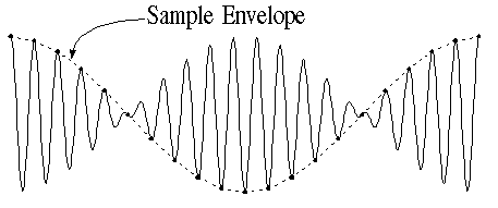
In the second situation, both inputs are high frequency signals but their frequencies are close to each other. The down-conversion of these closely placed frequencies can generate a slow-varying modulation envelope whose frequency is orders of magnitude lower than the input frequencies. For example, Figure 2-17 shows a down-conversion mixer where TD ENVLP analysis can be used to trace out the modulation envelope by choosing either of the fast varying signals as the clock. In general, you should choose as the clock signal the signal that causes the most nonlinearity. Be aware that single carrier HB ENVLP analysis does not handle this well because HB ENVLP treats signals other than the clock signal as DC signals in one cycle of the clock. Multi-carrier HB ENVLP can handle this case.

Figure 2-17 Down Conversion of Two Closely Placed Frequencies

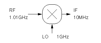
As is true for Periodic Steady-State (PSS) analysis, you can use ENVLP analysis for particular classes of circuits operating with multiple clock fundamentals. For PSS analysis, the multiple fundamentals are commensurate. For ENVLP analysis, you can use the greatest common denominator of all fundamental clock frequencies as the clock beat frequency. The process of selecting the clock beat frequency for ENVLP analysis is similar to the process of figuring out the beat frequency for PSS analysis. In similar situations where multiple clock fundamentals are present, ENVLP analysis is also analogous to PSS in terms of efficiency. Each time the clock period is integrated, a large number of fast cycles might be involved. The efficiency of the method depends on how many fast cycles occur per beat period. The more fast cycles you need to simulate, the less efficient the method. Because HB ENVLP regards the signals other than clock as DC signals, currently HB ENVLP is not a good choice to simulate a circuit with fast cycles other than clock. Multi-carrier HB Envelope should be used instead by either

Setting LO and RF as the fundamentals, and regarding IF as slow signals.
Regarding IF as a modulated wave, and setting LO, RF and IF as the fundamentals.

One difference between the ENVLP and PSS analyses is that for ENVLP analysis, you use a single clockname to identify the fundamentals. The simulator automatically calculates the beat frequency. For PSS analysis, you figure out the beat frequency either at the UI level or by entering it as an analysis parameter.

In a certain sense, an ENVLP analysis might be considered as a fast transient analysis whose efficiency comes from skipping simulation cycles. However, when an ENVLP analysis cannot find cycles to skip, the analysis effectively reduces to a transient analysis. Therefore, ENVLP analysis might not always be more efficient than transient analysis due to the greater computational overhead required for ENVLP analysis when it cannot find enough cycles to skip. Nevertheless, ENVLP analysis is always as accurate as PSS analysis.

ENVLP Parameters

For information on ENVLP analysis parameters, refer to the Envelope Following Analysis (envlp) section in the Spectre Circuit Simulator Reference manual.

The Envelope Choose Analysis form is similar to the transient Choose Analysis form. Most ENVLP analysis parameters are inherited from either transient or PSS analysis and their meanings are consistent. However, a few parameters need clarification.

The procedure for setting up an ENVLP analysis is similar to the set-up procedure for transient analysis. Important parameters for ENVLP analysis include: clockname, period, fund, funds, flexbalance, maxharms, harmonicbalance, harms, stop, envmaxstep, modulationbw, fixstepsize, swapfile, and fmspeedup.

The following list summarizes several important differences between ENVLP analysis and transient analysis. The parameter names are those used inside Spectre RF. For ENVLP analysis, do the following:

Identify a periodic, built-in source with the clockname parameter. This requirement is similar to QPSS analysis requirements. However, for ENVLP analysis, you need only name the clock source. You can select any periodic, built-in source (sine, pulse, or pwl) as the clock. The simulator examines all the sources whose name matches the clockname to determine the clock frequency. If more than one frequency is found, the greatest common factor of these frequencies is used as the clock frequency.
When applied to autonomous circuits, ENVLP analysis requires that you specify a pair of nodes, p and n, as for PSS analysis. You cannot use clockname for autonomous circuits. If the period of the carrier is known, period of fund could be set to get the clock frequency directly, and clockname is ignored.
To use multi-carrier HB Envelope, funds and maxharms must be provided, just like QPSS. Multi-carrier HB Envelope uses the QPSS HB engine and adopts the same parameters funds and maxharms.
If harmonicbalance is yes, HB Envelope is used. If it is no, TD Envelope is used. The default is no. For multi-carrier HB Envelope, this parameter is regarded as yes automatically.
Specify which harmonics of the clock frequency are of interest with the harms/harmsvec parameter. For TD Envelope, the default for harms is 1, which is appropriate for most applications. The number of harmonics you specify affects both output and computation time, but it does not affect accuracy. Hence, you should avoid specifying unnecessary harmonics. For example, in a power amplifier, only the first harmonic is needed because the signal of interest is near the fundamental frequency. In a mixer, both the zeroth and the first harmonics are needed because signals at both the baseband and near the fundamental frequency are of interest. For single carrier HB Envelope, the default for harms is 3. The number of harmonics does affect accuracy because HB Envelope calculates in frequency domain. For multi carrier HB Envelope, harms is replaced by maxharms. For multi-carrier HB Envelope, harmsvec also specifies the harmonics which need output, each group of elements with the size equal to that of funds is a selection of specific harmonic combinations of fundamental frequencies.
Specify a stop time long enough to detect slow signals. For example, complete at least a few clock cycles.
The maximum envelope step size is affected by many parameters. It can be directly limited by envmaxstep. It is helpful to specify a modulationbw frequency that reflects how the envelope is varying. This parameter provides an estimate of the modulation bandwidth and the simulator puts at least eight points within the modulation period. An approximate value is sufficient. To improve the noise floor in power spectrum density computation, use strobeperiod to get equally spaced envelope points.
If fixstepsize is yes, ENVLP analysis skips cycles indicated by stepsize. The efficiency of Envelope analysis depends on how many cycles are skipped. The strategy is designed for general situations. For some cases, Envelope is faster with an appropriate fixed stepsize.
Specify a swapfile for simulation of large circuits. The same requirement holds for PSS and QPSS analyses. The swapfile parameter is supported for only the shooting engine.
Specify fmspeedup=yes for circuits with frequency modulated input.

Most of the remaining parameter requirements are the same as for the Spectre RF transient (tran) analysis and their meanings are consistent.

The errpreset Parameter in ENVLP Analysis

The effect of errpreset on some particular ENVLP analysis parameters is shown in Table 2-6.

Table 2-6 Parameter Defaults as a Function of errpreset

errpreset	maxstep	envmaxstep	reltol	relref	steady ratio	envlteratio
`liberal`	T/20	`Interval/10`	`0.01`	`sigglobal`	`0.1`	`0.35`
`moderate`	T/20	`Interval/25`	`0.001`	`sigglobal`	`0.1`	`3.5`
`conservative`	T/50	`Interval/50`	`0.0001`	`alllocal`	`1.0`	`35.0`

The effect of errpreset on parameters such as reltol, relref, method, maxstep, and lteratio is the same as defined for transient analysis with one exception. The transient simulation interval in ENVLP analysis is always a clock period.

The default value for compression=no.

For compression=no, the output file stores data for every signal at every timepoint for which Spectre RF calculates a solution. Spectre RF saves the x axis data only once, because every signal has the same x value.
For compression=yes, Spectre RF writes data to the output file only when the signal value changes by at least twice the convergence criteria. To save data for each signal independently, x axis information corresponding to each signal must be saved.
- If the signals in your circuit stay at constant values for large periods of the simulation time, setting compression=yes results in a smaller output data file.
- If the signals in your circuit move around a lot, setting compression=yes results in a larger output data file.

ENVLP analysis generates two types of output files for each specified harmonic of the clock fundamental

A voltage versus time (td) file
An amplitude/phase versus time (fd) file

The td file contains real time-domain waveforms. This file is generated when outputtype={envelope, both}. The waveforms are similar to waveforms generated by Transient analysis. The difference between the two is that for ENVLP analysis the integration of a clock cycle is done occasionally. Consequently, you normally see gaps between integrated clock cycles. Note that multi-carrier HB Envelope analysis does not generate a td file.

The fd file contains time varying Fourier coefficients (complex) of the circuit response at clock harmonics. The fd file is generated when outputtype={spectrum, both}. Time varying Fourier coefficients are discussed in “ACPR Calculation”.

The actual spectrum of each harmonic response is calculated from the Analog Design Environment (ADE) GUI. This is useful for applications such as ACPR calculation.

Plotting the Results of ENVLP Analysis

The Envelope Following Direct Plot form plots

Three different waveform (or Function) types
- Voltage
- Current
- Power
Three sweep types
- Time
- Harmonic Time
- Spectrum.

As shown in Figure 2-18, waveforms are called Functions on the ENVLP analysis Direct Plot form.

Figure 2-18 A Typical ENVLP Direct Plot Form

Plotting Voltage vs Time Waveforms

When you select both a waveform (Signal) and the sweep type Time, you plot a cycle-sampled version of the waveform.

When you use an Amplitude Modulated (AM) example with a 1 GHz carrier and a 1 MHz baseband tone, the resulting plot is a sampled version of the AM waveform. Instead of taking a continuous set of points as a transient analysis would, the ENVLP analysis saves simulation time by taking intelligently spaced samples of the waveform. When you visually connect the tops of the waveform samples, you can see the envelope that results from an equivalent transient analysis.

Depending on the phase of the clock at which the sampling occurs, different time domain envelopes result. Figure 2-19 shows two envelopes that might result from sampling at different clock phases. Either envelope might be traced out by an ENVLP analysis.

Figure 2-19 Sample Envelopes

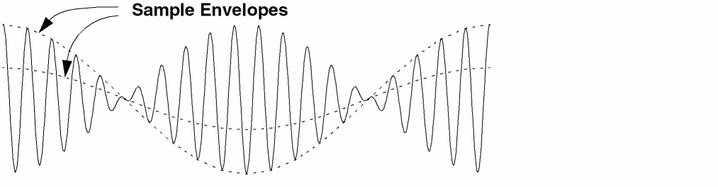
The other two sweep types (harmonic time and spectrum) plot voltage as a complex waveform. For complex waveforms, you can plot either the magnitude/phase or the real/imaginary parts of the waveform. Note that if you change the clock phase at which sampling occurs, these complex waveforms are not affected.

When you select both signal and harmonic time as the sweep type, you plot the complex, time-varying Fourier coefficient for each harmonic. Using the AM example, when you select the 1^st harmonic you see the 1 MHz baseband signal. In other words, the ENVLP analysis essentially strips off the 1 GHz carrier.

Plotting Power Spectral Density

When you select both signal and spectrum, the Power Spectral Density Parameter fields appear at the bottom of the plot form. After you provide values for the fields, the Direct Plot form calculates the total number of samples, window size, and number of bins, and then calls the psdbb calculator function.

Table 2-7 describes the Power Spectral Density Parameter fields.

Table 2-7 Power Spectral Density Parameters
From time and to time	Starting and ending times, respectively, for the time interval during which the spectral analysis is to be performed. Normally, these parameters are set to the simulator start and stop times, respectively. However, you might want to make the From time different than zero to exclude the start-up transient from the analysis. The Time Interval should be long enough to support the frequency resolution you want.
Nyquist half-bandwidth	Normally this parameter is set to 3 to 5 times the maximum modulation bandwidth frequency. The Nyquist half-bandwidth indirectly determines the spacing of the time points used in the FFT calculations. When the original time domain data points are too far apart to support the Nyquist bandwidth, you might see strange results such as unexpected spikes in the spectrum. The Nyquist half-bandwidth should be less than half the inverse of the smallest time step. To avoid aliasing, all signals in the system must have negligible power at the Nyquist half-bandwidth and beyond.
bin-width	The Frequency bin width determines the frequency resolution. A smaller frequency resolution usually produces a noisier spectrum. The power spectral density is a frequency-by-frequency average of the FFT taken over several time windows within the main time interval. A smaller Frequency bin width produces fewer samples to average together at each frequency. If you chose a small bin width, the resulting PSD looks “noisy” and has a jagged appearance. If you make the bin width too large you might soften what should be sharp edges in the spectrum.
Max plotting frequency and Min plotting frequency	The Min and Max plotting frequencies are the minimum and maximum frequency you wish to display. The Min plotting frequency is negative because the resulting plot is the power spectral density of a baseband signal. The power spectral density of a baseband signal does not necessarily have complex conjugate symmetry because the signal is generally complex.
windowing name	A preset list of available windowing functions used during the spectrum calculation. The Window selection determines how data at the edges of a time window is attenuated to control spectral leakage. Spectral leakage occurs because an FFT is always taken over a finite time interval. That is like multiplying the original waveform by a pulse of amplitude one and duration equal to the duration of the data. Multiplication in the time domain corresponds to convolution in the frequency domain. The transform of the long pulse is a high and narrow sinc function. As the pulse length goes to infinity, the main lobe of the sinc function approaches a Dirac delta function. When estimating the spectrum at a given frequency, the sinc function’s side lobes cause spectral components of the untruncated signal to leak into the estimation of the spectrum at the main lobe.
detrending	Allows you to remove certain trends from the data before the spectral analysis. The options are None, Mean and Linear. None means do not detrend Mean removes the mean Linear removes the linearly growing component

The following typical parameter settings are used for the AM example just mentioned. These numbers assume that the Stop time is set to 60 us:

`Start time`	0
`Stop time`	60us
`Nyquist half-bandwidth`	5e6
`Bin-width`	20e3
`Max plotting freq`	5e6
`Min plotting freq`	-5e6
`Windowing name`	hamming
`Detrending`	none

For the AM example, you see a waveform displayed as V ² / ( Hz ) versus frequency. You can think of this as

(rms passband volts) *   (rms passband volts) / Hz

The spectrum plot is the estimated power spectral density of the complex envelope divided by two. The division by two occurs because the envelope is in units of peak carrier volts but power in the carrier equals the square of the peak divided by two. It is convenient to express the envelope in peak units because it can then be directly compared against an input baseband signal.

The calculated total number of samples, window size, and bin-width are printed to the CIW (Command Interpreter Window) so you have the option of using the psdbb calculator function. As shown later, direct use of the psdbb function together with strobing can dramatically drop the noise floor. The following list displays the calculations that generate the psdbb parameters:

L =To - From (the To and From times are user inputs)
fmax (Nyquist half-bandwidth) and bin-width are user inputs
#bins = floor(L*binwidth) , compute with #bins >= 1 . Here, floor means take the integer part of..., or truncate to the nearest integer.
Compute the smallest m such that
2 ^m ∗ (#bins) > 2 ∗ L ∗ fmax
windowsize = 2 ^m
number of samples = #bins ∗ windowsize

AGC Example

One application of ENVLP analysis is to assess the Automatic Gain Control (AGC) loop dynamics. AGC loops are important in communication systems where wide amplitude variations in the output signal leads to a loss of information. These signals need a good control to maintain a constant signal level at the output.

The PSS and QPSS analyses cannot compute the AGC response because the response is not periodic. The loop might have a periodic response if it were unstable but PSS and QPSS would be difficult to apply because the period of the instability would not be known before running the simulation. Transient analysis is not usually a good choice because the frequencies of the amplitude oscillation and carrier are too far apart. ENVLP analysis is an efficient and accurate alternative for assessing the stability of AGC loops as this example shows.

Consider the AGC loop shown in Figure 2-20. The behavioral blocks are simple multipliers from the ahdl library. The upper left multiplier is the variable gain amplifier (VGA). After filtering, the amplitude detector produces the square of the amplitude of the VGA output. The AGC loop input is a fixed-amplitude 100 Mhz carrier. A stable version of this circuit would generate an output signal with the same phase as the input signal but with the amplitude determined by the feedback loop. This design has an extra integration in the feedback loop that makes the loop unstable. The simulator’s challenge here is to detect the design error by quickly and accurately simulating the unstable behavior.

Figure 2-20 AGC Loop

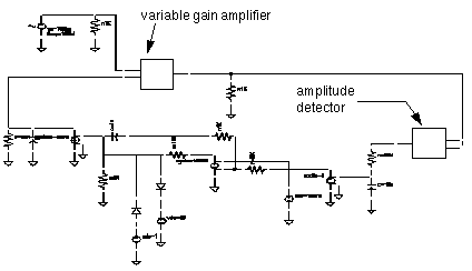
Figure 2-20 compares the results of transient analysis with the TD ENVLP and HB ENVLP analyses.

The common parameters for all three analyses are

Stop time=2m

Accuracy Defaults(errpreset)=moderate

For both ENVLP analyses

Number of harmonics=1

In Figure 2-21, waveforms for all three analyses show the instability in the output amplitude. Both ENVLP analyses (top) avoid a number of redundant carrier cycles and run much faster than the transient analysis (bottom). The TD ENVLP analysis is about 47 times faster than the transient analysis. The HB ENVLP analysis is 293 times faster than the transient analysis because this case is quite linear. The time savings is even greater with a 1 GHz carrier.

Figure 2-22 compares the ENVLP analyses with the transient analysis (bottom) for a single cycle. The ENVLP simulation is not only fast, it is accurate.

The Spectre RF workshop includes this example. It shows how to set up an envelope analysis for this case and how to see further results. Refer to the workshop for more information.

Figure 2-21 Comparison Between Transient and ENVLP Analyses Results

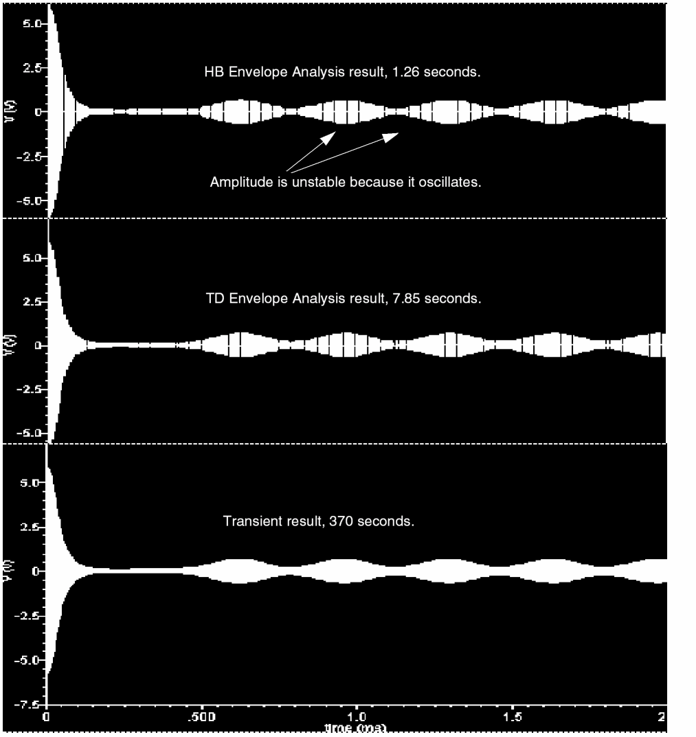
Figure 2-22 Blow-up of One ENVLP Cycle with the Transient Waveform

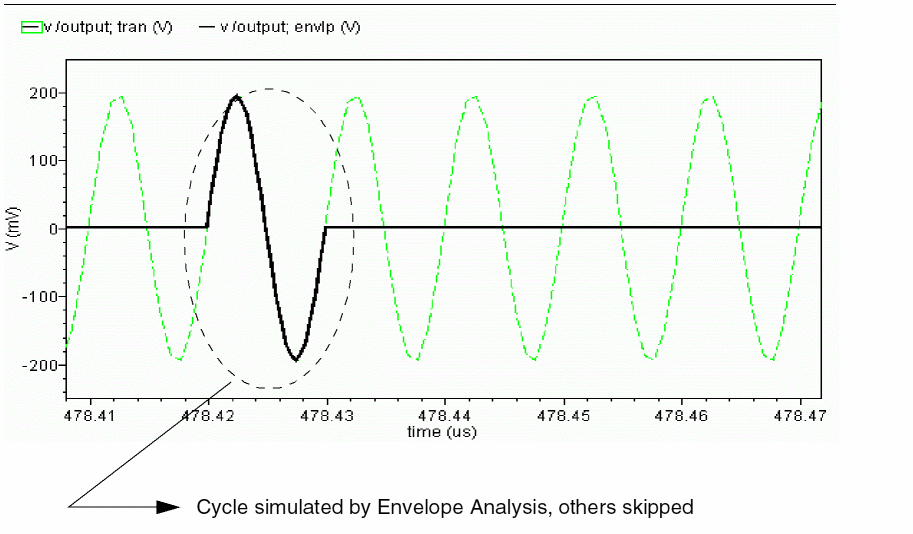
ACPR Calculation

ACPR (Adjacent Channel Power Ratio) is a common measure of how much power a transmitter emits outside its allotted frequency band. It is the ratio of the power in an adjacent band divided by the power in the allotted band. Regardless of exactly how you chose the frequencies and bands for the ACPR measurement, it is always extracted from the power spectral density of the transmitted signal. This section describes how the Analog Design Environment (ADE) estimates power spectral density (PSD).

You cannot compute the PSD directly from PSS and QPSS analyses because the input baseband signals carry information and are therefore not periodic. The J-model (see [5] for details) is a very fast indirect method for computing ACPR, but like all behavioral models, has limitations. Using an ENVLP analysis, you can check J-model ACPR calculations much faster than you can with transient analysis.

PSDs are always estimated because the information riding on the carrier is a stochastic process and the Fourier transform of a stochastic process is ill defined. No matter how you chose to define the spectral nature of a stochastic process, it must involve an averaging process. Any empirically derived average is an estimate because one can never take an infinite number of samples.

The PSD is a frequency-by-frequency average of a set of DFTs (discrete Fourier transforms) of the baseband signal. Here, the baseband signal is the harmonic-time result of an ENVLP analysis.

The waveform is first interpolated, if necessary, to generate evenly spaced data points in time. The spacing of the data points is the inverse of the DFT sampling frequency. The PSD is computed by first breaking the time Interval up into overlapping segments. Each segment is multiplied, time point by time point, by the specified Windowing function. Windowing reduces errors caused by a finite time record. It is impossible to work with an infinite time record. Direct use of an unwindowed finite time record is equivalent to multiplying the infinite record by a rectangular pulse that lasts as long as the data record. Multiplication in the time domain corresponds to convolution in the frequency domain. The Fourier transform of a rectangular pulse is a sinc function. Considering the frequency domain convolution, the side lobes of the sinc function cause parts of the true spectrum to leak into the frequency of interest, the frequency of the main lobe. Ideally, the sinc function would be a Dirac delta function but that requires an infinite time record. Good windowing functions have smaller side lobes than a sinc function.

The DFT is performed on each windowed segment of the baseband waveform. At each frequency, the DFTs from all segments are averaged together. Fewer segments means fewer data points in the average at a particular frequency. The length of each segment is inversely proportional to the Frequency bin width. This is why a small bin width produces a jagged PSD. A smaller bin width means a longer time segment. Fewer long segments fit into the given Time Interval so there are fewer DFTs to average together. In the extreme, there is only one segment and no averaging. Without averaging, the PSD is just the square of the magnitude of the DFT of a stochastic process. At the other extreme, large bin widths produce lots of points to average at each frequency but there are fewer frequencies at which to average because fewer large bins fit into the Nyquist frequency. The PSD is smoother but it does not have as much resolution.

A PSD Example

This section describes the various ENVLP outputs and how to use them to generate a PSD. Figure 2-23 shows the ACPR test circuit.

The behavioral blocks are two multipliers and one adder that model an ideal I/Q modulator
The carrier frequency is 1 GHz
The amplifiers are transistor-level models

The baseband input signals are read in with piecewise linear sources. The piecewise linear sources read data files. In this example, the data files contain CDMA baseband signals and are stored in the rfLib. The files are listed as cdma_2ms_idata and cdma_2ms_qdata. The stored signals were created with the CDMA signal generator, which is also in the rfLib. You cannot use the CDMA signal generator directly because its internal DSP filters have a hidden state. Spectre RF does not work with any AHDL model that has a hidden state. You can also generate the baseband signals with SPW. The piecewise linear sources also read SPW’s data format.

Figure 2-23 ACPR Test Circuit

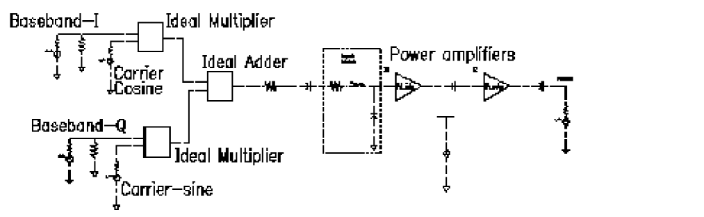
Figure 2-24 displays the time response of the RF output. The top picture shows some of the cycles. A number of cycles are missing. This illustrates why ENVLP analysis is faster than transient analysis.

Figure 2-24 ENVLP Analysis Time Response

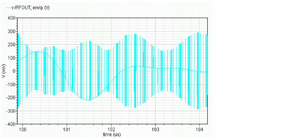
Although you can see something resembling an envelope in the time response, the detailed cycles can obscure it on larger time scales and it is not guaranteed to represent any particular phase of the envelope. The harmonic time response is designed to extract the baseband components or any other harmonic of interest. Most of the time the fundamental, or first harmonic, is the most interesting.

The harmonic analysis plots the real and imaginary parts of the specified Fourier component of each cycle as a function of its location in time. Figure 2-25 and Figure 2-26 show how the real and imaginary parts of the fundamental components of the RF input and output signals evolve with time. These signals are the baseband representations of the RF signals.

Figure 2-25 Input (top) and Output (bottom) Baseband Waveforms

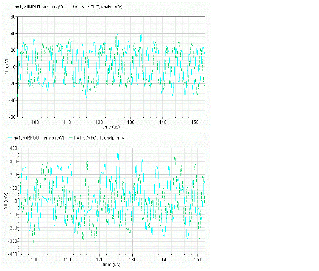
Not much can be ascertained directly from time-domain baseband waveforms. However, x-y plots of real and imaginary waveforms show the trajectory traced out by the baseband signal in the symbol constellation space. Figure 2-26 shows the input and output baseband trajectories. A trajectory is displayed by changing the x-axis to be the real waveform. The output trajectory is a scaled and rotated version of the input trajectory. The scaling factor is evident in the time domain waveforms but the trajectories also make the phase shift obvious. The transmitter introduces about 45 degrees of phase shift.

Figure 2-26 Baseband Input and Output Trajectories

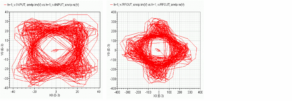
ACPR estimation requires power spectral densities. Use the spectrum button on the ENVLP Results form to estimate the power spectral density of a baseband signal. The baseband signal is the time-varying fundamental Fourier component described above. Figure 2-27 compares input and output power spectral densities. Because the input and output power spectral densities have the same shape, you can tell that this example shows very little spectral regrowth

Figure 2-27 Power Spectral Densities of the Input and Output RF Signals

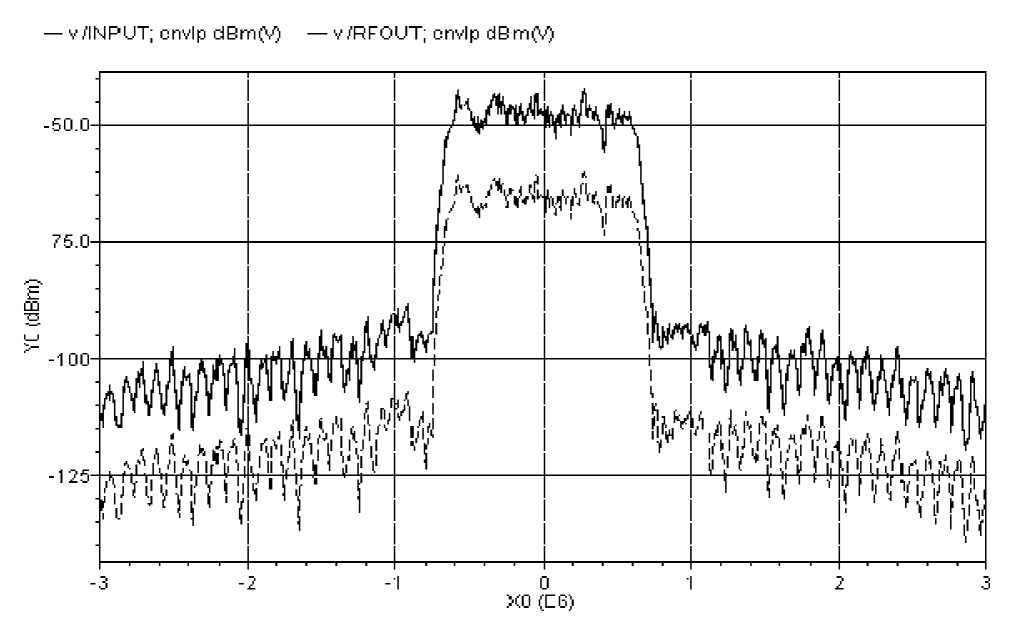
The power spectral densities shown in Figure 2-27 were created with the following option values.

From	0 s
To	300 us
Nyquist half-bandwidth	3 MHz
Frequency bin width	10 KHz
Max. plotting frequency	3 MHz
Min plotting frequency	-3 MhZ
Window	Hanning
Detrending	None

The baseband signal driving the transmitter dominates the transmitted PSD. In most cases, the baseband signals come from digital filters and the digital filters constrain the spectrum of the input baseband signal. Distortion in the transmitter causes the spectrum to grow where it should not, hence the need for an ACPR measurement. In measuring ACPR it is crucial to drive the transmitter with the proper baseband signals.

It is not practical to model digital filters in Spectre RF because Spectre RF cannot simulate state variables inside Verilog-A modules. Consequently, for now, you must pre-compute and store the baseband inputs and read them into the Spectre RF analysis through the ppwlf sources found in the analogLib, as shown in this example. The ppwlf sources also read SPW format, so you can also generate and record the input baseband waveforms using SPW.

The rfLib contains three sets of stored baseband waveforms, cdma, dqpsk, and gsm. These waveforms were created with the baseband signal generators in the measurement category of the rfLib.

If you want to measure ACPR with the noise floor much more than 40dB below the peak of the output power spectral density, you need to create baseband drive signals with a noise floor at or below the required noise floor. If you use a DSP tool like SPW to create the signals, the filters in the baseband signal generator have to operate perhaps hundreds of times faster than those in the actual generator. Otherwise the signals do not have enough resolution. The noise floor depends heavily on interpolation error. You can strobe the harmonic time results to eliminate interpolation of the output but you can not eliminate interpolation of the baseband drive signals. The only way to reduce interpolation errors at the input is to use ultra-high resolution drive signals so that no matter where the interpolation occurs, the error is small. It is up to the user to generate ultra-high resolution drive signals.

The Fourier analysis used to compute the power spectral density uses evenly spaced time points. If data does not exist at one of the Fourier time points, the Fourier algorithm must interpolate to create it.

The Spectre RF workshop includes this example. To see how to setup envelope analysis for this case or to get further information, see the workshop.

Validation

A practical transmitter circuit [6] was simulated using the ENVLP analysis. The circuit has 185 MOSFETs, 79 nodes and 127 equations. It is driven by a 1.7475 GHz carrier and GSM baseband signals. The transient behavior was simulated for 2.5 ms, or roughly 4.5 million carrier cycles. It would take traditional transient analysis 154 days to simulate on an UltraSparc 10 with a 299 MHz CPU and generate 10 GB of data. In contrast, it took the ENVLP analysis 17.5 hours to finish in the same computing environment and it generated 1.2 MB of data. More importantly, the ACPR calculation from the ENVLP analysis results matched very well with measured data as shown in Figure 2-28. The two results diverge past about 400 KHz but that is irrelevant to ACPR in this case because GSM channels are only 200 KHz wide.

Figure 2-28 ACPR Simulation Results

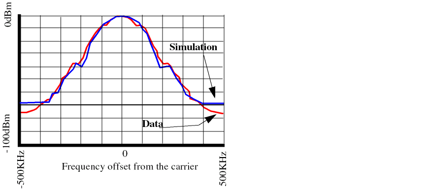
Autonomous ENVLP Analysis

RF circuits used in communication systems make great demands on the accuracy and efficiency of simulators. This is especially true when a strongly nonlinear circuit operates at high-frequency oscillating modes and contains slowly time-varying driving sources.

Circuits exhibiting these characteristics include

A PLL with time-varying reference
An RF mixer with a local oscillator
An AGC plus VCO
An oscillator followed by a power amplifier (PA)

Usually, the dynamics of these circuits involve multiple time scales and frequency-modulated (FM) signals. In these circuits, the fast time-scale oscillating frequency is modulated by slow time-scale signals.

Because transient analysis is very expensive for circuits with multi-rate dynamics, Cadence uses various envelope technologies to speed up the simulation. Traditional TD ENVLP analysis is efficient for non-autonomous circuits with AM, PM, FM or mixed modulated signals. However, in the FM case, if the modulation index is large, the signal spectrum contains Bessel functions that are distributed in a wide frequency range. Standard ENVLP analysis does not handle this situation accurately and efficiently. Furthermore, ENVLP analysis requires a fixed frequency so it cannot handle the unknown frequencies of oscillator circuits. On the other hand, periodic steady-state analyses, such as HB PSS, can be used to simulate oscillator circuits but they do not allow any time-varying sources in the circuit.

The autonomous ENVLP analysis combines ENVLP analysis and autonomous steady-state PSS analysis. In this form of analysis, the oscillator problem is solved for each slow-varying time step. Then, the slow-varying characteristics of the circuit (including instantaneous oscillating frequencies and other envelope information) is obtained by integrating occasional cycles.

A Faster Steady State Oscillator Analysis

In the steady state (PSS) oscillator analysis, the initial values specified for oscillating frequency and other conditions are important for Newton convergence. To estimate the value of the stabilized frequency, a transient analysis can be performed before the steady state oscillator analysis. In some oscillator circuits, such as high Q circuits, it takes a long time for the oscillation to build up and stabilize. In this case, autonomous envelope can be used to speed up the analysis.

Figure 2-29 The rfOsc Oscillator Schematic

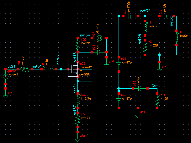
For the rfOsc example shown in Figure 2-29, the oscillator takes about 1.5 microseconds to start up and 3.5 microseconds to stabilize. The results are shown in Figure 2-30.

Use the following analysis commands to speed up the PSS analysis.

Do enough microseconds of autonomous ENVLP analysis to ensure the oscillation is stable and write the solution into the env.dat file.
Do an autonomous PSS analysis that skips the DC analysis and reads the initial condition from the env.dat file.
Do a Pnoise analysis and calculate the phase noise for the oscillator.

Example 2-1 illustrates the three analysis statements.

Example 2-1 Analysis Commands for a Faster PSS Analysis

envlp (Out 0) envlp harms=3 stop=20u maxstep=100p envmaxstep=100n flexbalance=1
+ tstab=2u fund=400M method=traponly envmethod=traponly errpreset=moderate
+ annotate=status writefinal="env.dat"

pss  (  Out 0 )  pss  fund=410M  harms=10 skipdc=yes readic="env.dat"
+ annotate=status  tstabenvlp=no

pnoise  (  Out  )  pnoise  sweeptype=relative relharmnum=1 start=1K stop=300M
+ dec=5 maxsideband=10  annotate=status

To run autonomous ENVLP analysis efficiently

To use HB Envelope, flexbalance must be set to yes. Otherwise, TD Envelope is used. If flexbalance is yes, harms is the maxharms of the clock fundamental and the default value is 3. The harms is an output parameter for TD but it is an input parameter for HB. Consequently, harms has a significant impact on the performance.
A reference port, for example, (Out 0), must be specified to indicate autonomous. This is similar to autonomous PSS. The reference port is used for two purposes:
- Estimating the initial fundamental frequency and calculating instantaneous frequencies at each envelope time step.
- Checking the phase=0 condition for the port when doing shooting or HB Newton iterations.
The reference port for ENVLP and the reference port for PSS can be different. For a better estimate of the period, select one of the output ports of an oscillator whose output waveform is close to sinusoidal.
In a non-autonomous envelope analysis (but not in an autonomous analysis), the clockname must be specified. However, in an autonomous envelope analysis, the fund or period option must be specified as an initial guess of the fundamental frequency.
Usually, you must set a tstab value. The default value of tstab for an autonomous envelope analysis is 4 cycles of the fundamental, which might not be enough to ensure convergence. During an HB Envelope analysis, especially for high-Q designs, enough tstab is needed to ensure that the oscillation starts.
Sometimes tightening the reltol parameters for the HB autonomous envelope analysis can make the result more accurate at the calculated cycle, which might improve the prediction and allow more cycles to be skipped. However, do not set reltol tighter than 1e-6 because that decreases the performance dramatically.

The oscillating frequency is 410 MHz, which corresponds to the period 2.44 nanoseconds. Figure 2-30 shows that there are about 0.1 microseconds between two occasional ENVLP analysis cycles. This implies that about 40 cycles were skipped for each ENVLP analysis step.

Figure 2-30 Autonomous ENVLP Analysis Results over 20 Microseconds

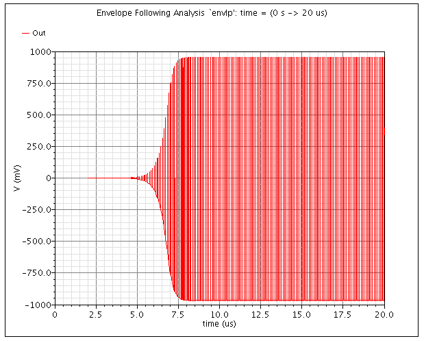
Figure 2-31 Transient Analysis Results over 20 Microseconds

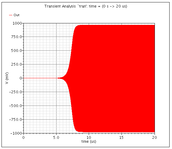
After the autonomous ENVLP analysis, you can plot the time-varying instantaneous frequency. For example, applying a 1 MHz sinusoidal source on the control voltage of a 3.46 GHz VCO circuit and then displaying the instantaneous frequency produces the plot shown in Figure 2-32. The ripple on the curve indicates that the VCO frequency follows the 1 MHz modulation signal. This circuit cannot be analyzed using either autonomous PSS or non-autonomous ENVLP analysis. The transient analysis can be used but it is very time consuming as discussed in the previous example.

Figure 2-32 Instantaneous Frequency of VCO with Sinusoidal Control Voltage

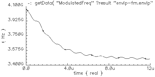
Simulating a Mixer with a VCO

This example simulates a mixer with two inputs

Baseband data
Output from the VCO circuit (LO)

The results show that the VCO frequency is affected by the baseband data signal.

Figure 2-33 is the circuit schematic for the example. The details of the VCO are not shown in the schematic. Figure 2-34 and Figure 2-35 show the modulation effects to oscillating frequency from a sinusoidal and a digital data input of port Prf respectively.

Figure 2-33 Schematic of Mixer with VCO

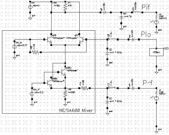
Figure 2-34 Results with Sinusoidal Data at Prf

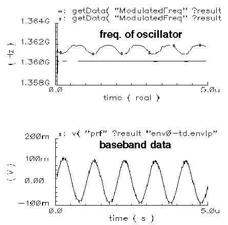
Figure 2-35 Results with Digital Data at Prf

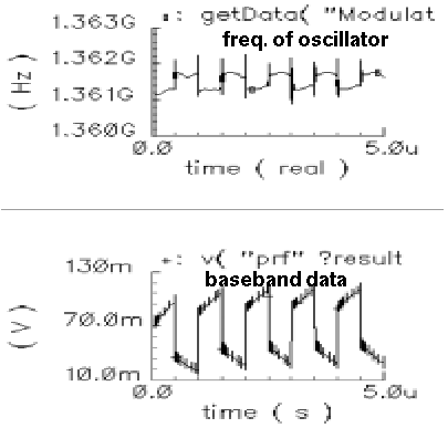
Simulating Oscillator-Pulling Effects for a Power Amplifier

In oscillator design, the oscillator-pulling effect is a common problem that can degrade performance. LO pulling is a phenomenon in which the LO frequency is influenced by a strong power amplifier signal when both the power amplifier output and the oscillator are at a high frequency.

This example simulates the system whose block diagram is shown in Figure 2-36. The system contains a local oscillator and a mixer followed by two power amplifier stages.

Figure 2-36 Circuit to Measure the Load Pulling Effect for an Oscillator

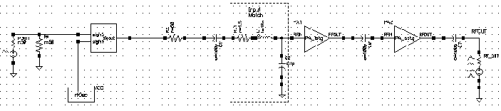
The simulation results are plotted in Figure 2-37. The upper plot is the instantaneous frequency from the VCO output. The lower plot is the baseband data signal. The figure shows that the oscillating frequency is affected by the power amplifier.

Figure 2-37 Simulation Results Showing Pulling Effect of the Oscillator

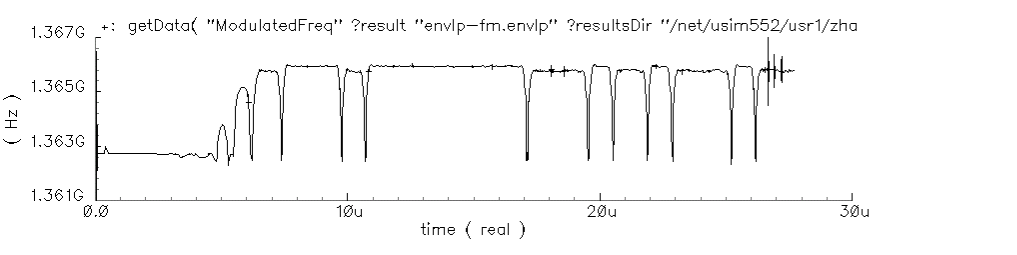
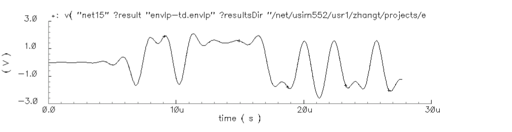
Simulating Circuits with Driven FM Sources

Another new feature of ENVLP analysis is faster simulation for circuits with driven FM sources.

Standard envelope analysis handles FM signals by sampling the signal at equal interval time points. The period is determined by the carrier frequency. For FM signals with large modulation indexes, standard envelope analysis is

Not efficient due to Newton iteration failures. The failures occurs because the polynomial condition is not satisfied. This can be seen in Figure 2-38 and Figure 2-39. Figure 2-38 indicates that standard envelope analysis is not working at all and the simulator is just doing a transient analysis.
Not accurate for computing the harmonic coefficients, which have been defined as the envelopes of the signal, because the real instantaneous frequency is different from the frequency used to do the Fourier transform. This can be seen by examining the output results of post-processing in Figure 2-40 and Figure 2-41, which display the derivative of phase for the first harmonic for the two methods respectively.
Figure 2-38 Standard ENVLP Analysis for an FM Signal

Figure 2-39 Faster ENVLP Analysis for an FM Signal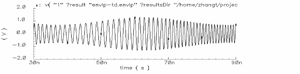

Figure 2-40 Frequency Profile Output From the Standard Method

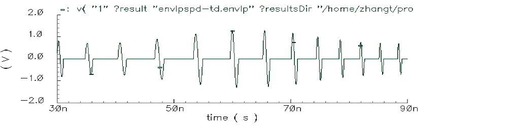Figure 2-41 Frequency Profile Output From Fast ENVLP Analysis for FM Sources

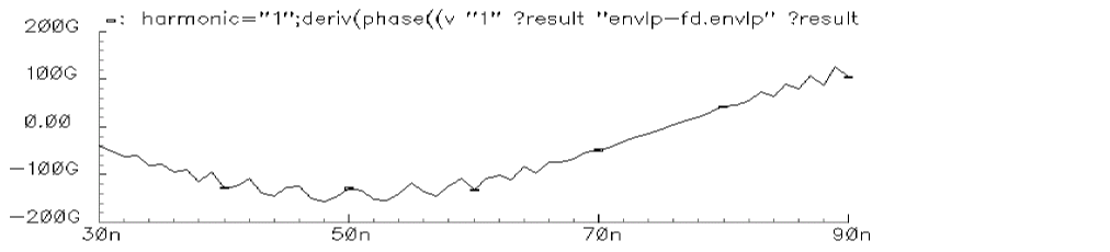
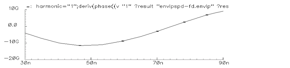
To use the fast ENVLP analysis, you must represent the FM driven sources with Spectre internal source models such as the port, vsource, and isource components. Then, set the ENVLP analysis option fmspeedup=yes.

Arbitrary Frequency Modulated Sinusoidal Sources

FM sinusoidal sources can be specified in three different ways using vsource, isource, or port.

Specify modulated frequency (sinusoidal modulation)
```
V1 (1 2) vsource type=sine freq=ω₀ fmmodindex=k fmmodfreq=ω
```
For this case, write the FM signal from the source as

Specify one file name, where the file contains the FM data
```
V1 (1 2) vsource type=sine freq=ω₀ fmmodindex=k fmmodfiles=[“f_data”]
```
For this case, write the FM signal from the source as

where δω(τ) is the frequency modulation data from the f_data file.

Specify the names of two files that contain I and Q data for modulation. For example,
```
V1 (1 2) vsource type=sine freq=ω₀ fmmodindex=k fmmodfreq=[“I” “Q”]
```
For this case, write the FM signal from the source as

Here, k is the modulation index

Where I(t) and Q(t) are the data from the I and Q files, respectively.

The file format for the I and Q files is the same as the PWL file format. The keywords related to PWL files (such as pwldbm and pwlperiod) also work for FM files in this case.

Running a Fast FM ENVLP Analysis

To speed up the FM ENVLP analysis, set the fmspeedup=yes option in the ENVLP analysis command. The default value of fmspeedup=no. Also set clockname to be the same as the fundname of the FM source.

Notice that the fast FM ENVLP analysis has the following limitations.

The algorithm that speeds up the ENVLP solver only works with FM sources
Frequency modulation can be applied only to sinusoidal sources (type=sine)

The following schematic, shown in Figure 2-42, is a circuit that includes an FM source followed by a PA, an LNA, and several other receiver components that perform demodulation.

Figure 2-42 The Circuit with an FM Source

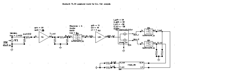
The FM source V ₁ is defined as follows

V1 (net22 0) vsource type=sine ampl=180.00m freq=2.442G \

fmmodindex=24420000 fundname="f_carrier" fmmodfiles=[ "f_data" ]

With fmspeedup=0, ENVLP analysis runs for 140 s for this case. The result at net22 is shown in Figure 2-43. With fmspeedup=1,ENVLP analysis runs for 27.8 s. The result at net22 is shown in Figure 2-44.

Figure 2-43 Output at net22 From Standard ENVLP Analysis

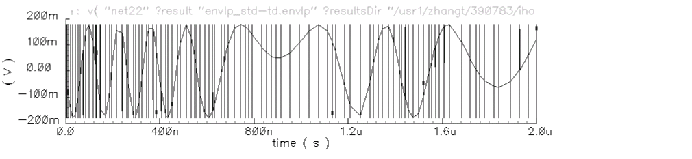
Because the clock frequency is adjusted while fmspeedup=1, the phase of each clock cycle is constant. Hence, a straight trace line is shown in Figure 2-44. However, with fmspeedup=0, the phase of each clock cycle is changing, which is shown in Figure 2-43.

Figure 2-44 Output at net22 From ENVLP Analysis with fmspeedup=1

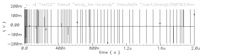
Frequently Asked Questions

Is ENVLP analysis as fast as transient analysis?

For circuits without hidden states, (which are usually introduced by Verilog-A modules), the answer is yes. Because a Newton method similar to that of PSS is used in Envelope analysis, circuits with hidden state cause difficulties, just as they do for PSS. However, most hidden states can be overcome [10].

How do I choose which ENVLP analysis to use?

The HB method is very efficient when simulating weakly nonlinear circuits because only a few harmonics are needed to represent the solution accurately. For highly nonlinear circuits with sharply raising or falling signals, time domain shooting is more suitable. However, when exploring design trade-offs using a few harmonics where accuracy is not of primary concerns, HB envelope might be the best choice.

How should I choose the number of harmonics for HB ENVLP analysis?

The default value is 3. The best value to use depends on the linearity in one cycle of the fast signal (LO or clock). For linear cases, a value of 1 is enough for accurate results. However, for nonlinear cases, such as a circuit with a square clock, even a value of 15 might not be large enough.

For what kind of circuits is multi-carrier HB Envelope suited?

As its name suggests, multi-carrier HB envelope analysis is designed for circuits with multi-carrier signals. For example, in a modulation system with a 1G LO and 10M IF where IF is a modulated signal, both LO and IF can be looked on as carriers, so multi-carrier HB Envelope is useful.

Does multi-carrier HB Envelope support the function FM speed up?

No, it does not.

Does multi-carrier HB Envelope handle autonomous circuits?

No, it does not. Multi-carrier HB Envelope uses the multi-tone HB engine, which does not handle autonomous circuits.

References

[1]	R. Telichevesky, K. Kundert and J. White. “Efficient steady-state analysis based on matrix-free Krylov-subspace methods”. Proceedings of the 32nd Design Automation Conference, June 1995.
[2]	D. Feng, J. Phillips, K. Nabors, K. Kundert and J. White, “Efficient computation of quasi-periodic circuit operating conditions via a mixed frequency/time approach”. Proceedings of the 36th Design Automation Conference, June 1999.
[3]	L. Petzold, “An efficient numerical method for highly oscillatory ordinary differential equations”. SIAM Journal of Numerical Analysis, vol. 18, no. 3, pp 455-479, June 1981.
[4]	K. Kundert, J. White and A. Sangiovanni-Vincentelli. “An envelope-following method for the efficient transient simulation of switching power and filter circuits”. IEEE International Conference on Computer-Aided Design: Digest of Technical Papers, November 1988.
[5]	J. Chen, D. Feng, J. Phillips, and K. Kundert, “Simulation and modeling of intermodulation distortion in communications circuits”. Proceedings of the Custom Integrated Circuit Conference, San Diego, CA, May 1999.
[6]	K. C. Tsai and P. R. Gray, “A 1.9GHz 1W CMOS class E power amplifier for wireless communications”, IEEE Journal of Solid State Circuits, pp. 962-970, Jul. 1999.
[7]	Behzad Razavi. RF Microelectronics, Prentice Hall, c1998. Series: Prentice-Hall Communications Engineering & Emerging Technologies Series.
[8]	E. Ngoya, J. Rousset, and D. Argollo. “Rigorous RF and microwave oscillator phase noise calculation by envelope transient technique”. In Microwave Symposium Digest, 2000 IEEE MTT-S International, volume 1, pages 91-94 vol.1, 2000.
[9]	O. Narayan and Jaijeet Roychowdhury, Analyzing Oscillators Using Multitime PDEs.
[10]	Ken Kundert, Hidden State in SpectreRF, 2003.

lteratio=10.0 for conservative errpreset. Only if user-specified reltol <= 1e-4 * 10.0/3.5, lteratio is set to 3.5.

* : lteratio=10.0 for conservative errpreset by default. Only if user-specified reltol <= 1e-5*10.0/3.5, lteratio is set to 3.5..

* : lteratio=10.0 for conservative errpreset by default. However, when the specified reltol

<= 1e-5*10.0/3.5, lteratio is set to 3.5..

Return to top

Spectre Circuit Simulator RF Analysis TheoryProduct Version 23.1, June 2023

2

The Spectre RF Analyses

Periodic Steady-State Analysis (PSS)

The Shooting Method

Parameters for PSS Analysis

The PSS Algorithm for Driven and Autonomous Circuits

Driven PSS Analysis

The Initial Transient Phase of PSS Analysis

Table 2-1 Timing Intervals for PSS Analysis

The Shooting Phase

Autonomous PSS Analysis

Phases of Autonomous PSS Analysis

Increasing the tstab Interval

Simulation Accuracy Parameters

Plotting the Current Spectrum

The High-Order and Finite Difference Refinement Parameters

Table 2-2 The relref Parameter Options

The errpreset Parameter in PSS Analysis

Using the errpreset Parameter With Driven Circuits

Table 2-3 Default Values and Noise Floor for errpreset in Driven Circuits

Using the errpreset Parameter With Autonomous Circuits

Table 2-4 Default Values and maxstep for errpreset in Autonomous Circuits

Other Parameters

Periodic AC Analysis (PAC)

PAC Synopsis

Intermodulation Distortion Computation

Frequency Sweep

Modulated Small-Signal Analyses

Sampled Small-Signal Analysis

Parameters for PAC Analysis

Periodic S-Parameter Analysis (PSP)

PSP Synopsis

Parameters for PSP Analysis

Periodic Transfer Function Analysis (PXF)

Parameters for PXF Analysis

Output Parameters

Probe Parameters

Output Parameters

Modulation Parameters

Sampled Small-Signal Analysis

Swept PXF Analysis

Periodic Noise Analysis (Pnoise)

Pnoise Synopsis

Parameters for Pnoise Analysis

Noise Figure

Frequency-Aware PPV Analysis for Oscillators with Large Time Constants

Flicker Noise

Flicker Noise Spectrum

Periodic Stability Analysis (PSTB)

Parameters for PSTB Analysis

Sweep

Understanding Loop-Based and Device-Based Algorithms

About the PSTB Loop-Based Algorithm

Device-Based Algorithm

Quasi-Periodic Steady-State Analysis (QPSS)

Comparing QPSS Analysis with PSS and PAC Analyses

QPSS Parameters

The errpreset Parameter in QPSS Analysis

Table 2-5 Parameter Default Values for errpreset Settings

Quasi-Periodic Noise Analysis (QPnoise)

QPnoise Output

QPnoise Synopsis

Swept QPnoise Analysis

QPnoise Parameters

Quasi-Periodic AC Analysis (QPAC)

QPAC Output Frequency and Sideband Vectors

Swept QPAC Analysis

QPAC Parameters

Quasi-Periodic S-Parameter Analysis (QPSP)

QPSP Output Frequencies and Sideband Vectors

Input and Output Frequencies in QPSP

Noise Analysis with QPSP

Noise Folding Effects

Swept QPSP Analysis

QPSP Parameters

Quasi-Periodic Transfer Function Analysis (QPXF)

QPXF Output Frequencies and Sideband Vectors

Transfer Function Inputs

Swept QPXF Analysis

Spectre Circuit Simulator RF Analysis Theory
Product Version 23.1, June 2023

Table 2-3 Default Values and Noise Floor for `errpreset` in Driven Circuits

Table 2-4 Default Values and maxstep for `errpreset` in Autonomous Circuits

Table 2-5 Parameter Default Values for `errpreset` Settings