rfJc

rfJc(
[ ?result t_result ]
[ ?resultsDir t_resultsDir ]
[ ?unit t_unit ]
[ ?ber g_ber ]
[ ?from n_from ]
[ ?to n_to ]
[ ?k n_k ]
[ ?multiplier n_multiplier ]
)
=> n_value / o_waveform / nil

Description

Calculates cycle jitter from the results of hbnoise or pnoise sample (jitter) analysis.

Arguments

?result t_result	Name of the result of Pnoise sample analysis.
?resultsDir t_resultsDir
	Path to the results directory.
?unit t_unit	Unit of jitter measurement. Valid values are ppm, Second, and UI.
?ber g_ber	Value of bit-error rate (BER) when the signal level is peak-to-peak.
?from n_from	The lower frequency limiter.
?to n_to	The upper frequency limiter.
?k n_k	Number of cycles, which determines whether one period or k-periods jitter are calculated. The default value is 1, which indicates that only one cycle jitter is calculated.
?multiplier n_multiplier
	Frequency multiplier. The default value is 1.

Value Returned

n_value	Value of cycle jitter if simulation is run in single run mode.
o_waveform	Waveform of cycle jitter if simulation is run in sweep mode.
nil	Result name is not correct or cycle jitter cannot be calculated because of an error.

Examples

The following example opens simulation results of hbnoise analysis stored in the specified results directory.

openResults("/home/user/hbnoise/lib/cell/view/results/maestro/ExplorerRun.0/1/test/psf")

=> "/home/user/hbnoise/lib/cell/view/results/maestro/ExplorerRun.0/1/test/psf"

The following example lists the results available in the currently open results directory.

results()

(hb_fi hb_fd hb_td hbnoise hbnoise_am

    hbnoise_pm hbnoise_lsb model instance output

    designParamVals primitives subckts variables

)

The following example selects the hbnoise_pm result from the current results directory.

selectResults('hbnoise_pm)

=> stdobj@0x315b06f8

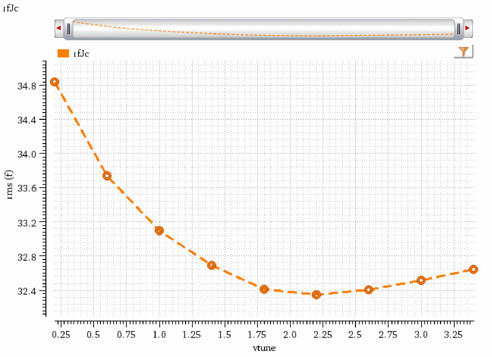
The following example creates a waveform object wave1 in which sweep variable is plotted on x axis and jitter value is plotted on y axis. The signal level is rms.

wave1=rfJc(?from 10K ?to 1G ?k 1 ?multiplier 1 ?result "hbnoise_pm" ?unit "Second")

=> srrWave:0x3574fbc0

The following example creates a Waveform window and returns its window ID.

win1=awvCreatePlotWindow()

=> window:3

The following example plots the waveform wave1 in the Waveform window win1.

awvPlotWaveform(

    win1

    list(wave1)

    ?expr list("rfJc")

    ?color list("y6")

    ?lineType list("line")

    ?lineStyle list("dash")

    ?lineThickness list("thick")

    ?showSymbols list(t)

    ?dataSymbol list("o")

    )

=> t

Note that the sweep variable vtune is plotted on x axis and jitter values are plotted on y axis.

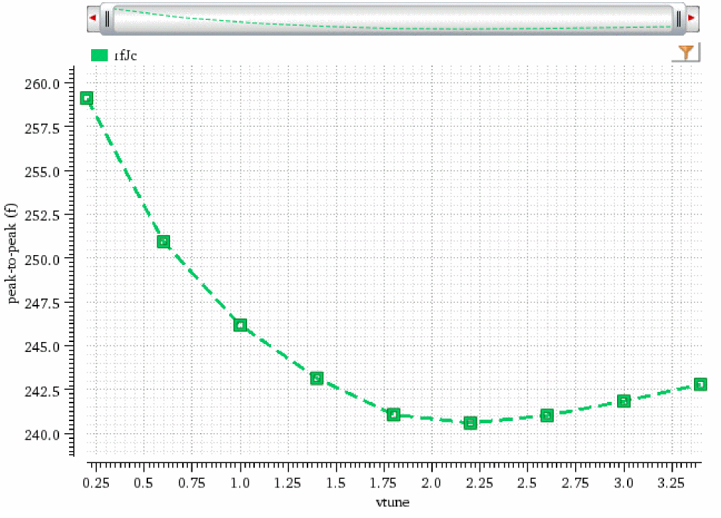
The following example creates a waveform object wave2 in which sweep variable is plotted on x axis and jitter value is plotted on y axis. The signal level is peak-to-peak and BER is 1e-4.

wave2=rfJc(?from 10K ?to 1G ?k 1 ?multiplier 1 ?result "hbnoise_pm" ?unit "Second" ?ber 1e-04)

=> srrWave:0x3574e7a0

The following example creates a Waveform window and returns its window ID.

win2=awvCreatePlotWindow()

=> window:4

The following example plots the waveform wave2 in the Waveform window win2.

awvPlotWaveform(

    win2

    list(wave2)

    ?expr list("rfJc")

    ?color list("y18")

    ?lineType list("line")

    ?lineStyle list("dash")

    ?lineThickness list("thick")

    ?showSymbols list(t)

    ?dataSymbol list(5)

    )

=> t

Note that the sweep variable vtune is plotted on x axis and jitter values are plotted on y axis.

The following example opens simulation results of pss_pnoise analysis stored in the specified results directory.

openResults("/servers/user/testcase/simulation/lib/cell/view/results/maestro/ExplorerRun.0/1/pss_pnoise_trannoise/psf")

=> "/servers/user/testcase/simulation/lib/cell/view/results/maestro/ExplorerRun.0/1/pss_pnoise_trannoise/psf"

The following example lists the results available in the currently open results directory.

results()

(pss_tran pss_td pss_fd pnoise_sample_pm0 model

    instance output designParamVals primitives subckts

    variables

)

The following example selects the result pnoise_sample_pm0 stored in the results directory.

selectResults('pnoise_sample_pm0)

=> stdobj@0x324df290

The following examples calculate values of cycle jitter from the result pnoise_sample_pm0 in units UI, Second, and ppm, respectively. The signal level is rms.

rfJc(?from 2.5K ?to 19.2M ?k 1 ?multiplier 1 ?result "pnoise_sample_pm0" ?unit "UI")

=> 5.02066e-06

rfJc(?from 2.5K ?to 19.2M ?k 1 ?multiplier 1 ?result "pnoise_sample_pm0" ?unit "Second")

=> 1.307463e-13

rfJc(?from 2.5K ?to 19.2M ?k 1 ?multiplier 1 ?result "pnoise_sample_pm0" ?unit "ppm")

=> 5.02066

The following examples calculate values of cycle jitter from the result pnoise_sample_pm0 in units UI, Second, and ppm, respectively. The signal level is peak-to-peak and BER is 1e-12.

rfJc(?from 2.5K ?to 19.2M ?k 1 ?multiplier 1 ?result "pnoise_sample_pm0" ?unit "UI" ?ber 1e-12)

=> 7.063566e-05

rfJc(?from 2.5K ?to 19.2M ?k 1 ?multiplier 1 ?result "pnoise_sample_pm0" ?unit "Second" ?ber 1e-12)

=> 1.83947e-12

rfJc(?from 2.5K ?to 19.2M ?k 1 ?multiplier 1 ?result "pnoise_sample_pm0" ?unit "ppm" ?ber 1e-12)

=> 70.63566

Return to top