RNM is a mixed approach, borrowing concepts from analog and digital simulation domain. The values are continuous, floating-point (real) numbers, as in the analog world. However, time is discrete, implying that the real signals change values based on discrete events. In this approach, we apply the signal flow concept so that the digital engine can solve the RVM system without support of the analog solver. This ensures high simulation performance in the range of a normal digital simulation and orders of magnitudes higher than the analog simulation speed.
The following lists the simulation performance, accuracy, and modeling effort, for the analog subsystem, common levels of abstraction:
- Extracted transistor netlist including parasitic elements
- Post layout representation
- Highest level of accuracy that can be achieved in circuit-level simulation
- Huge amount of devices
- Low simulation performance
- Transistor-level representation,
- SPICE-level simulation
- Nominal reference for analog simulation
- Often used as “golden” simulation reference
- Fast SPICE simulation
- Trade off between accuracy and speed
- Mostly close to SPICE-level simulation accuracy
- Simulation speedup compared to classical SPICE in the range of 20x
- SPICE-level simulation
- Analog behavioral modeling
- Conservative behavioral models using voltages and currents
- Written in Verilog-A, Verilog-AMS, or VHDL-AMS
- Typical speedup compared to classical SPICE in the range of 5-100x
- Real Nummber modeling
- Continuous value, discrete time (event-based) models
- Signal flow models
- Written in Verilog-AMS, VHDL, SystemVerilog, e
- Maintaining analog-like behavior
- Can be solved in digital simulation kernel
- Simulation performance close to digital speed
- Compared to classical SPICE approach, a performance improvement of 100000-1000000x can be achieved
- Pure digital model
- Digital model for analog blocks
- Written in Verilog, SystemVerilog, and VHDL
- Analog signal represented as single logic value: very poor representation of analog behavior but potentially sufficient for connectivity type of checks
- Analog signal represented as logic bus: similar accuracy as RVM, however, no match between digital and analog implementation (bus vs. scalar wire)
The gain in simulation performance and reduction in accuracy are highly dependent on the application. There is no general recommendation on what level of abstraction might be useful. This heavily depends on the verification goals
Additionally, RVM opens up the possibility of connecting with other advanced verification technologies, without the difficulty of interfacing with the analog engine or defining new semantics to deal with the analog values, such as:
- Assertion-based verification
- Metric-driven verification (randomization, coverage, and assertion-based)
- Higher-level verification languages, such as SystemVerilog and e
The following figure shows a general trend in the accuracy/performance tradeoff. The numbers are generic and can vary significantly for different applications.
Figure 1.1: Model Accuracy Versus Performance Gain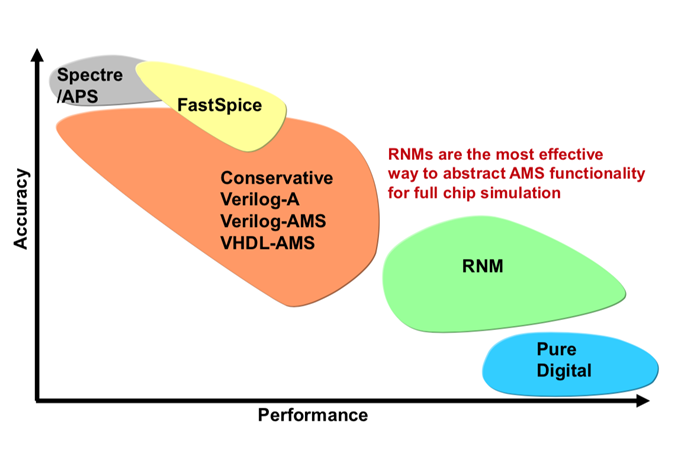
Classical SPICE-level simulations are used as golden reference simulation. Fast SPICE engines reach the same accuracy but can also trade-off some accuracy for speed (mainly fast SPICE). Analog behavioral modeling provides a large range of capabilities, reaching from high accuracy to high performance. However, it should be noted that a low-performance, low- accuracy model is a potential risk for inexperienced modelers. In particular, convergence issues caused by over-idealized models might slow down the overall simulation significantly. This may result in a performance decrease rather than the expected simulation speed improvement.
As mentioned earlier, RVM provides high simulation performance but restricts the model accuracy at the same time. Finally, pure digital model can be very inaccurate but might be sufficient for verification tasks including connectivity checks.
The following figure illustrates the general trends in the effort required to set up a simulation or create the model.
Figure 1.2: Model Accuracy Versus Performnace Gain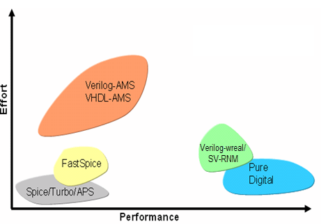
As SPICE simulations are reference simulations, these are always executed and the effort to run this simulation must always be taken into account. Turbo SPICE and APS setup require only one additional option (+aps); so no additional work is required. Since FastSpice simulations require a detailed control on speed vs. accuracy, on a block-level basis, some amount of setup effort and understanding of the design is required.
Analog behavioral model creation effort can range from hours to days and possibly weeks to become a good behavioral model. RNM is inherently restricted to the signal flow approach and analog convergence is not an issue. Consequently, the modeling effort is significantly lower as compared to analog behavioral models. More importantly, the design engineer does not need to learn a new language to create real number models. Therefore, the ramp-up time to create these models is much lower than creating analog behavioral models. On the other hand, pure digital models – not using RNM – do have significant drawbacks in terms of functionality that limit the use for analog models.
Behavioral models can also be differentiated by the modeling goal. A performance-oriented model needs to precisely capture critical behavior, which is necessary to efficiently explore the design space and make implementation trade-offs. Functional models capture the actual circuit behavior only to the detail needed to verify the correct design functionally. Both types of models are found in top-down and bottom-up modeling. However, the top-level functional verification is far more common in bottom-up modeling where it is used to perform the final design verification prior to tape-out. For example, the functional verification model can be used to study dynamic closed-loop functionality between the RF and digital baseband ICs, whereas a performance-oriented model of an RF block can be used for cascaded measurements, such as IP3 and explore system-level metrics, such as bit error rate and error vector magnitude.