2
Creating Modules
A module definition appears between the keywords module and endmodule or macromodule and endmodule. The following definition for a digital to analog converter illustrates the form of a module definition.
See the following topics for information about creating and using modules in Cadence® Verilog®-AMS:
- Declaring Modules
- Declaring the Module Interface
- Specifying Supply Sensitivity Attributes
- Defining Module Analog Behavior
- Using Internal Nodes in Modules
-
Chapter 10, “Instantiating Modules and Primitives”
This chapter contains detailed discussions about declaring and connecting ports and about instantiating modules.
Declaring Modules
To declare a module, use this syntax.
module_declaration ::=
module_keywordmodule_identifier[ ( list_of_ports ) ] ; [ module_items ] endmodule
module_keyword ::=
        module
 |   macromodule
module_items ::=
        { module_item }
    |   analog_block

module_item ::=
        module_item_declaration
    |   parameter_override
    |   module_instantiation
    |   digital_continuous_assignment
    |   digital_gate_instantiation
    |   digital_udp_instantiation
    |   digital_specify_block
    |   digital_initial_construct
    |   digital_always_construct
module_item_declaration ::=
        parameter_declaration
    |   aliasparam_declaration
    |   input_declaration
    |   output_declaration
    |   inout_declaration
    |   ground_declaration
    |   integer_declaration
    |   net_discipline_declaration
    |   real_declaration
    |   genvar_declaration
    |   branch_declaration
    |   analog_function_declaration
    |   digital_function_declaration
    |   digital_net_declaration
    |   digital_reg_declaration
    |   digital_time_declaration
    |   digital_realtime_declaration
    |   digital_event_declaration
    |   digital_task_declaration
parameter_override ::=
        defparam list_of_param_assignments ;
|
An ordered list of the module’s ports. For details, see “Ports”. |
|
Declaring the Module Interface
Use the module interface declarations to define
For example, the module interface declaration
module res(p, n) ;
inout p, n ;
electrical p, n ;
parameter real r = 0 ;
declares a module named res, ports named p and n, and a parameter named r.
Module Name
To define the name for a module, put an identifier after the keyword module or macromodule. Ensure that the new module name is unique among other module, schematic, subcircuit, and model names, and any built-in Spectre® circuit simulator primitives. If your module has any ports, list them in parentheses following the identifier.
Ports
To declare the ports used in a module, use port declarations. To specify the type and direction of a port, use the related declarations described in this section.
list_of_ports ::=
         port { , port }

port ::=
         port_expression
    |    .port identifier( [port_expression ])
port_expression ::=
         port_identifier
    |    port_identifier [ constant_expression ]
    |    port_identifier [ constant_range ]

constant_range ::=
    msb_constant_expression : lsb_constant_expression
For example, these code fragments illustrate possible port declarations.
module exam1 ; // Defines no ports
module exam2 (p, n) ; // Defines 2 simple ports
Normally, you cannot use Q as the name of a port. However, if you need to use Q as a port name, you can use the special text macro identifier, VAMS_ELEC_DIS_ONLY, as follows.
`define VAMS_ELEC_DIS_ONLY
`include "disciplines.vams"
(module 1, which uses a port called Q)
(module 2, which use a port called Q)
...
`include "disciplines.vams"
(module 3, which uses an access function called Q)
(module 4, which uses an access function called Q)
...
This macro undefines the sections in the disciplines.vams file that use Q, making it available for you to use as a port name. Consequently, when you need to use Q as an access function again, you need to include the disciplines.vams file again.
module exam5 (.b(p), .d(n))  // Defines the ports b and d, which are
                             // connected to the signals p and n,
                             // respectively
Port Type
To declare the type of a port, use a net discipline declaration in the body of the module. If you do not declare the type of a port, you can use the port only in a structural description. In other words, you can pass the port to module instances, but you cannot access the port in a behavioral description. Net discipline declarations are described in “Net Disciplines”.
Ports declared as vectors must use identical ranges for the port type and port direction declarations.
Port Direction
You must declare the port direction for every port in the list of ports section of the module declaration. To declare the direction of a port, use one of the following three syntaxes.
input_declaration ::= input [ range ] list_of_port_identifiers ;
output_declaration ::= output [ range ] list_of_port_identifiers ;
inout_declaration ::= inout [ range ] list_of_port_identifiers ;
range ::= [constant_expression:constant_expression]
-
input: Declares that the signals on the port cannot be set, although they can be used in expressions. -
output: Declares that the signals on the port can be set, but they cannot be used in expressions. -
inout: Declares that the port is bidirectional. The signals on the port can be both set and used in expressions.inoutis the default port direction.
Ports declared as vectors must use identical ranges for the port type and port direction declarations.
In this release of Verilog-AMS,
-
The compiler does not enforce correct application of
input,output, andinout. - You cannot use parameters to define constant_expression.
Port Declaration Example
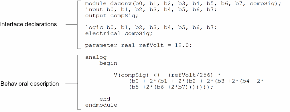
Module daconv, described below, has nine ports. The compSig port is declared with a port direction of output, so that its value can be set. The other ports are declared with a port direction of input, so that their values can be read. The compSig port is declared as an analog port of the electrical discipline.
module daconv(b0, b1, b2, b3, b4, b5, b6, b7, compSig); // Declares nine ports
input b0, b1, b2, b3, b4, b5, b6, b7;        // Declares ports as input
output compSig;                              // Declares port as output

logic b0, b1, b2, b3, b4, b5, b6, b7;        // Declares type of digital ports
electrical compSig;                          // Declares type of analog port

parameter real refVolt = 12.0;

analog
    begin

        V(compSig) <+  (refVolt/256) *(b0 + 2*(b1 + 2*(b2 + 2*(b3 +2*(b4 +2*
            (b5 +2*(b6 +2*b7)))))));

    end
endmodule
Parameters
With parameter (and dynamicparam) declarations, you specify parameters that can be changed when a module is used as an instance in a design. Using parameters lets you customize each instance.
For each parameter, you must specify a default value. You can also specify an optional type and an optional valid range. The following example illustrates how to declare parameters and variables in a module.
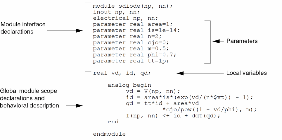
Module sdiode has a parameter, area, that defaults to 1. If area is not specified for an instance, it receives a value of 1. Similarly, the other parameters, is, n, cjo, m, phi, and tt, have specified default values too.
Module sdiode also defines three local variables: vd, id, and qd.
For more information about parameter declarations, see “Parameters”.
Specifying Supply Sensitivity Attributes
Add the groundSensitivity and supplySensitivity attributes to a port or pin definition in a mattributesodule to make a connect module sensitive to supplies in the module to which it connects.
sensitivity_attribute ::=
        (* [ integer groundSensitivity = "gSig_sensitive_to" ; ]
       [ integer supplySensitivity = "sSig_sensitive_to" ; ] *)
gSig_sensitive_to, sSig_sensitive_to
Names of signals, typically global signals, to which you want a connect module to be sensitive.
When you specify a supplySensitivity or a groundSensitivity attribute on a signal in a connect module, the declared signal (in the connect module) takes on the value of the supplySensitivity or groundSensitivity signal you specify.
When you specify a supplySensitivity or the groundSensitivity attribute (or both) on a signal in an ordinary module, the value of the supplySensitivity or groundSensitivity signal overrides the value of the signal of the same name in the connect module to which the ordinary module connects.
For example, you might use the groundSensitivity attribute in a connect module (such as l_to_e, below) as follows:
connectmodule l_to_e(dval, aval);
    ...
    electrical (* integer groundSensitivity = "global_pwr.pow1" ; *) gnd ;
    ...
endmodule
The default value of gnd in this connect module is the value of signal global_pwr.pow1. If module l_to_e connects to digital port d in ordinary module sample (below), the value of global_pwr.pow5, which appears in the groundSensitivity attribute for d, overrides the default value of gnd in the connect module.
module sample(d);
    output (* integer groundSensitivity = "global_pwr.pow5" ; *) d ;
    ...
endmodule
If port d does not have a groundSensitivity attribute, the value of gnd in the connect module retains its default value of global_pwr.pow1:
module sample(d);
    output d ;
    ...
endmodule
Making a connect module sensitive to supplies in the connected digital port is more likely to produce the behavior you expect because:
- When a connect module converts analog signals to digital values, the decision to output a one or a zero depends on the relationship between the analog signal and a threshold value. The software determines the threshold value based on the supply values in the component that includes the connected digital port.
- When a connect module converts digital values to analog signals, the connect module needs to determine what voltage to produce for each digital input value. Again, that voltage depends on the supplies in the component that includes the connected digital port.
The following basic principles apply to using these sensitivity attributes:
-
The software inserts connect modules between a digital port and an analog net. When you use the
groundSensitivityandsupplySensitivityattributes, you make the connect module sensitive to the signals on the digital port, regardless of the port direction. -
There are two steps involved in establishing ground or supply sensitivity: Specifying the necessary attributes in the connect module and adding the corresponding attributes to the connected digital port definition in the ordinary module.
- You must use detailed discipline resolution or the sensitivity attributes have no effect.
See the following topics for more information:
- Using the Sensitivity Attributes in a Chain of Buffers
- Using Sensitivity Attributes with Inherited Connections
Using the Sensitivity Attributes in a Chain of Buffers
Consider a design containing three buffers, such as the following, where buffers ba1 and ba3 are analog blocks with analog input and output pins, and buffer bd2 is a digital block with logic input and output pins:
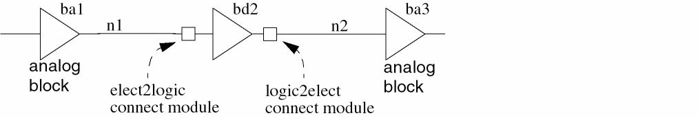
During elaboration, the software inserts connect modules across net n1 and the digital input port of buffer bd2, and across the digital output port of buffer bd2 and net n2.
If you know this design has an operating voltage of 5.0 Volts, you might write an analog-to-digital connect module with hard-coded thresholds, such as the following:
‘include "disciplines.vams"
connectmodule elect2logic(aVal, dVal);
    output dVal;
    input aVal;
    logic dVal;
    electrical aVal;
    reg temp;
    always begin              // Digital, do this always
    if(V(aVal) >  3.0)
        #1 temp = 1;          // Delay 1 time unit, drive output 1
    else if (V(aVal) < 2.0)
        #1 temp = 0;          // or drive output 0, depending on aVal
    else
        #1 temp = 1’bx;
    end
    assign dVal = temp;        // Bind register to digital output
endmodule
However, if the design can operate at 3.0 or 5.0 Volts depending on the supplies, you might use the supplySensitivity and groundSensitivity attributes to write a connect module that is sensitive to the supplies, such as the following:
// Supply-sensitive connect module
‘include "disciplines.vams"
connectmodule elect2logic(aVal, dVal);
    output dVal;
    input aVal;
    logic dVal;
    electrical aVal;
    electrical (* integer supplySensitivity = "cds_globals.\\vdd! " ; *) \vdd! ;
    electrical (* integer groundSensitivity = "cds_globals.\\vss! " ; *) \vss! ;
    reg temp;
    always begin                   // Do this always
    if(V(aVal) >  ((V(\vdd! ) - V(\vss! ))/2 + 0.5 ))
        #1 temp = 1;               // Delay 1 time unit, drive output 1
    else if (V(aVal) < ((V(\vdd! ) - V(\vss! ))/2 -0.5))
        #1 temp = 0;               // or drive output 0, depending on aVal
    else
        #1 temp = 1’bx;
    end
    assign dVal = temp;             // Bind register to digital output
endmodule
The threshold values are functions of the supply and ground values.
To specify the digital ports to which the connect module is sensitive, add groundSensitivity and supplySensitivity attributes to the connected digital port. In our example, the software inserts a connect module both at the input and at the output port of buffer bd2, so in the supply-sensitive module definition, you would add both sensitivity attributes to both ports of the buffer, like this:
module bux2_5V (Z,A);
input
    (* integer supplySensitivity="\\vdd! ";
       integer groundSensitivity="\\vss! "; *)
A ;
output
    (* integer supplySensitivity="\\vdd! ";
       integer groundSensitivity="\\vss! "; *)
Z;
wire \vss! ;
wire \vdd! ;
analog begin
    V(\vss! ) <+ 0.0 ;
    V(\vdd! ) <+ 5.0 ;
end
buf #1 (Z,A);
specify
    specparam
    t_A_Z_rise = 0.1,
    t_A_Z_fall = 0.1;
    // Delays
    (A +=> Z) = (t_A_Z_rise,t_A_Z_fall);
endspecify
endmodule
Using Sensitivity Attributes with Inherited Connections
An inherited connection is a net expression associated with either a signal or a terminal. You use inherited connections to override specific global names in your design. For more information, see “Inherited Connections” in the Virtuoso Schematic Editor L User Guide.
You can use inherited connections to set the values of signals on ports and use the supply sensitivity attributes to make a connect module sensitive to those values. By doing so, you can switch between different power supplies (that you set by inherited connections) and have connect modules that behave differently depending on the value of the supplies.
For example, here is a buffer module with both supply sensitivity attributes on both the input and the output ports (A and Z). The signal name for each of the sensitivity attributes is an inherited connection (\\vdd! for supplySensitivity and \\vss! for groundSensitivity). The inh_conn_prop_name and inh_conn_def_value attributes on wires \vss! and \vdd! set the value of the inherited connections:
module bux2 (Z,A);
input
    (* integer supplySensitivity="\\vdd! ";
       integer groundSensitivity="\\vss! "; *)
A ;
output
    (* integer supplySensitivity="\\vdd! ";
       integer groundSensitivity="\\vss! "; *)
Z;
wire
    (* inh_conn_prop_name="lSup", // if set, specifies value for \vss!
        inh_conn_def_value="cds_globals.\\vss! " *)
\vss! ; // \vss! has default value cds_globals.\\vss!
wire
    (* inh_conn_prop_name="hSup", // if set, specifies value for \vdd!
       inh_conn_def_value="cds_globals.\\vdd! " *)
\vdd! ; // \vdd! has default value cds_globals.\\vdd!
buf #1 (Z,A);
‘ifdef functional
‘else
specify
    specparam
    t_A_Z_rise = 0.1,
    t_A_Z_fall = 0.1;
    // Delays
    (A +=> Z) = (t_A_Z_rise,t_A_Z_fall);
endspecify
‘endif
endmodule
You can compare this buffer module with module bux2_5V in the previous section, where the \vss! and \vdd! net values do not depend on inherited connections:
wire \vss! ;
wire \vdd! ;
The supply-sensitive connect module is the same as the one that appears in the previous section.
Defining Module Analog Behavior
To define the analog (continuous time) behavioral characteristics of a module, you create an analog block. The simulator evaluates all the analog blocks in the various modules of a design as though the blocks are executing concurrently.
analog_block ::=
        analog analog_statement

analog_statement ::=
    analog_seq_block
   |analog_branch_contribution
   |analog_indirect_branch_assignment
   |analog_procedural_assignment
   |analog_conditional_statement
   |analog_for_statement
   |analog_case_statement
   |analog_event_controlled_statement
   |system_task_enable
   |statement

statement ::=
    seq_block
   |procedural_assignment
   |conditional_statement
   |loop_statement
   |case_statement
analog_statement can appear only within the analog block.
statement can appear anywhere within the module, including within the analog block.
See “Sequential Block Statement” for more information about analog_seq_block and seq_block.
In the analog block, you can code contribution statements that define relationships among analog signals in the module. For example, consider the following contribution statements:
V(n1, n2) <+ expression;
I(n1, n2) <+ expression;
where V(n1,n2) and I(n1,n2) represent potential and flow sources, respectively. You can define expression to be any combination of linear, nonlinear, algebraic, or differential expressions involving module signals, constants, and parameters.
The modules you write can contain at most a single analog block. When you use an analog block, you must place it after the interface declarations and local declarations.
Because the description in the analog block is a continuous-time behavioral description, you must not use blocking event control statements, such as blocking delays, events, or waits, within the block.
The following module includes an analog block and initial and always blocks. These blocks work together within a single module to define an analog to digital converter.
module adc;
electrical vin;
parameter real a_amp = 5;        // This parameter is used by analog.
parameter real d_volt_range = 5; // This parameter is used by digital.
real a_freq, a_phase;
real d_half_range;
real d_vin;
real a_vin
real d_vin_save;
reg [7:0] b;

integer ii;
integer d_fd;
initial begin
        b = 0;
        d_half_range = d_volt_range / 2;
        d_fd = $fopen("ms6.dat");
        $fstrobe(d_fd,"time\tb\td_vin\ta_vin\n");
        d_vin = 0;
end
always begin
        #1;
        d_vin =  V(vin);          // Probes the voltage.
        d_vin_save = d_vin;

        for (ii=0; ii < 8; ii = ii + 1) begin // Converts the voltage into
                                              // an 8-bit register.
                if (d_vin > d_half_range) begin
                        b[ii] = 1;
                d_vin = d_vin -  d_half_range;
                end else b[ii] = 0;
                d_vin = d_vin * 2;
        end
        // Writes the digital output to a file.
        $fstrobe(d_fd,"%g\t%b\t%g\t%g",$abstime, b, d_vin_save, a_vin);
end
analog begin
      @(initial_step) begin
                a_freq = 10K;
      end

      // input
      a_phase = 2*‘M_PI*a_freq*$abstime;
      a_vin = a_amp*sin(a_phase);
      V(vin) <+ a_amp*sin(a_phase);     // Creates a sinusoidal voltage source.
end

endmodule
Defining Analog Behavior with Control Flow
You can also incorporate conditional control flow into a module. With control flow, you can define the behavior of a module in regions.
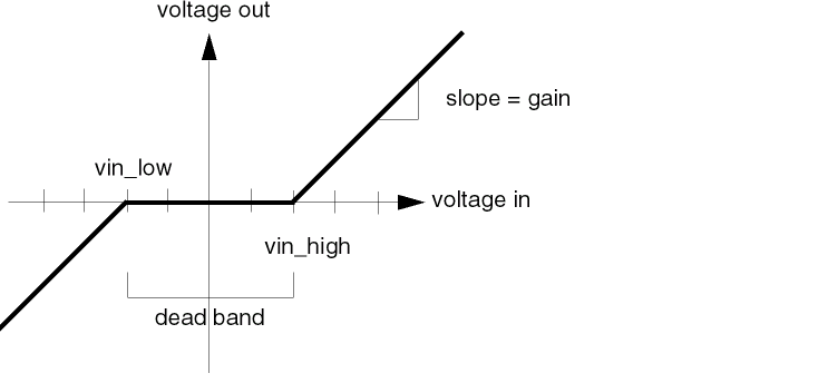
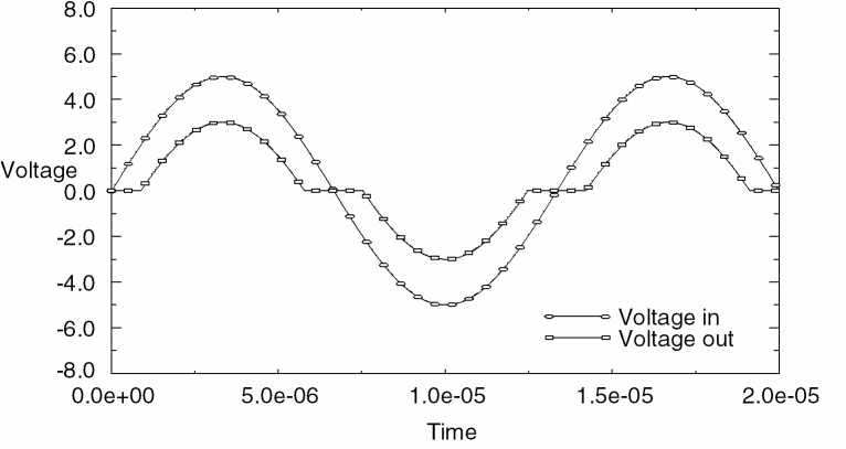
The following module, for example, describes a voltage deadband amplifier vdba. If the input voltage is greater than vin_high or less than vin_low, the amplifier is active. When the amplifier is active, the output is gain times the differential voltage between the input voltage and the edge of the deadband. When the input is in the deadband between vin_low and vin_high, the amplifier is quiescent and the output voltage is zero.
module vdba(in, out);
input in ;
output out ;
electrical in, out ;
parameter real vin_low = -2.0 ;
parameter real vin_high = 2.0 ;
parameter real gain = 1 from (0:inf) ;
 analog begin
      if (V(in) >= vin_high) begin
           V(out) <+ gain*(V(in) - vin_high) ;
      end else if (V(in) <= vin_low) begin
           V(out) <+ gain*(V(in) - vin_low) ;
      end else begin
           V(out) <+ 0 ;
      end
 end
endmodule
The following graph shows the response of the vdba module to a sinusoidal source.
Using Integration and Differentiation with Analog Signals
The relationships that you define among analog signals can include time domain differentiation and integration. Verilog-AMS provides a time derivative function, ddt, and two time integral functions, idt and idtmod, that you can use to define such relationships. For example, you might write a behavioral description for an inductor as follows.
module induc(p, n);
inout p, n;
electrical p, n;
parameter real L = 0;
 analog
      V(p, n) <+ ddt(L * I(p, n)) ;
endmodule
In module induc, the voltage across the external ports of the component is defined as equal to the time derivative of L times the current flowing between the ports.
To define a higher order derivative, you must use an internal node or signal. For example, module diff_2 defines internal node diff, and sets V(diff) equal to the derivative of V(in). Then the module sets V(out) equal to the derivative of V(diff), in effect taking the second order derivative of V(in).
module diff_2(in, out) ;
input in ;
output out ;
electrical in, out ;
electrical diff ;    // Defines an internal node.
 analog begin
      V(diff) <+ ddt(V(in)) ;
         V(out) <+ ddt(V(diff)) ;
    end

endmodule
For time domain integration, use the idt or idtmod functions, as illustrated in module integrator.
module integrator(in, out) ;
input in ;
output out ;
electrical in, out ;

    analog begin
         V(out) <+ idt(V(in), 0) ;
    end

endmodule
Module integrator sets the output voltage to the integral of the input voltage. The second term in the idt function is the initial condition.
Using Internal Nodes in Modules
Using Verilog-AMS, you can implement complex designs in a variety of different ways. For example, you can define behavior in modules at the leaf level and use the top-level module to define the structure of the system. You can also define structure within modules by defining internal nodes. With internal nodes, you can directly define behavior in the module, or you can introduce internal nodes as a means of solving higher order differential equations that define the network.
Using Internal Nodes in Behavioral Definitions
Consider the following RLC circuit.
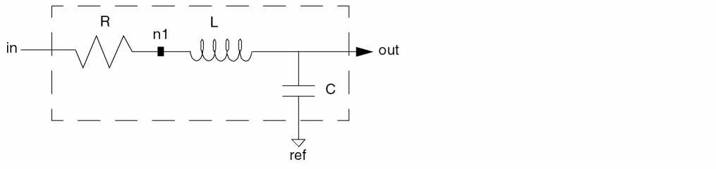
Module rlc_behav uses an internal node n1 and the ports in, ref, and out, to define directly the behavioral characteristics of the RLC circuit. Notice how n1 does not appear in the list of ports for the module.
module rlc_behav(in, out, ref) ;
inout in, out, ref ;
electrical in, out, ref ;
parameter real R=1, L=1, C=1 ;

    electrical n1 ;

    analog begin
         V(in, n1) <+ R*I(in, n1) ;
         V(n1, out) <+ L*ddt(I(n1, out)) ;
         I(out, ref) <+ C*ddt(V(out, ref)) ;
    end

endmodule
Using Internal Nodes in Higher Order Systems
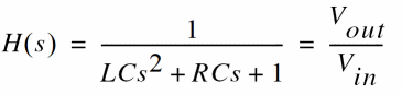
You can also represent the RLC circuit by its governing differential equations. The transfer function is given by
In the time domain, this becomes
Module rlc_high_order implements these descriptions.
module rlc_high_order(in, out, ref) ;
inout in, out, ref ;
electrical in, out, ref ;
parameter real R=1, L=1, C=1 ;

    electrical n1 ;

    analog begin
         V(n1, ref) <+ ddt(V(out, ref)) ;
         V(out, ref) <+ V(in) - (R*C*V(n1) - L*ddt(V(n1))*C ;
    end

endmodule
Return to top